External Memory Algorithms

The External Memory (EM) model of computing has been proposed to allow for the design of data structures and algorithms that are efficient for problems where the size of the data being processed exceeds the internal memory available to process the problem. In the EM model, algorithms are designed to process blocks of data in a manner that minimizes the need to read data from external memory to the computer's internal memory. The R-tree index is an example of such a data structure.

Notation

This section provides details on terminology conventions that will be used throughout this report, it is based on the conventions used for describing EM algorithms.

Assume we have some search problem, the basic parameters that can be used to evaluate the efficiency of a solution are as follows:

• N - the number of objects in the problem
• M - the number of objects fitting into main memory
• B - the number of objects stored in a single disk block
• T - number of objects reported by a query

For batch queries we also have

• K - number of queries in a batched query

A common convention in the external memory literature is to use the lower case volue of these iterms to represent the corresponding sizes in the number of blocks, such that,

• $n = N/B$
• $m = M/B$
• $t = T/B$
• $k = K/B$

Definition 1   A batch query is a query in which K queries are executed on a object set V where we are interested in the total time to answer all K queries. Batched queries can be classified as batched static queries where V is assumed to be static, or as batched dynamic queries which can involve a mix of insertions, deletions and queries and where query evaluation requires that the insertions and deletions be accounted for.

EM Batched Geometric Queries

The earliest attempt to apply EM algorithms to batch queries for geometric data structures was that of [13] where several external memory techniques are presented with application to computational geometry. These techniques are applied to the following geometric query problems.

• answering K range queries on N points in 1D
• answering K point location queries in a planar subdivision of size N
• pairwise intersections of the union of N rectangles

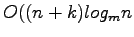
Solutions to each of these problems are presented which can be answered in $O( (n+k)\lg_{m}n + t)$ by applying the techniques of distribution sweeping, and batch filtering, where $K$ simultaneous external memory serachs are performed in data structures that can be modelled as planar layer directed acyclic graphs (DAGs). Where the problem instance involves no specific queries then assume $k=0$ and $t=1$ . The general approach of the distribution sweeping and batch filtering are presented in the following sections.

Distribution Sweeping

Distribution Sweeping is provides an I/O efficient implementation for main-memory algorithms that employ the commonly used plane sweep technique. The problem input is first sorted using an I/O efficient sorting method and then divided into m strips, each containing an equal number of input objects. When the 'sweep' step is performed the strips are scanned simultaneously from top to bottom, looking for componenents of the solution that involve interactions between objects in different strips. By using m strips we are ensured that a block of main-memory can be used for each strip. After between-strip components are found the within-strip components are found by recursively applying distribution sweep to each strip. The recursion requires $O(log_{m}n/m)$ levels at which point the subproblems are small enough to fit into main memory.

Orthogonal Line Segment Intersection

The operation of the distribution sweeping technique is most easily demonstrated through an example, which is given here in the form of the orthogonal line segment intersection problem. The problem can be defined as follows; Given a set of N orthogonal line segment report all K interesections between them. Assuming the segments are parallel to the x and y axes the technique involves the following steps.

1. Sort segment endpoints by x and y coordinates into two seperate lists.
2. Use the 'x' sorted list to split the input into $\lfloor m \rfloor$ vertical strips $\gamma_i$ . The y sorted list is then used in the top to bottom sweep. Associated with each vertical strip is an Active List, $A_i$ , which is a stack. A single block from each of the $\lfloor m \rfloor$ active lists is kept in main-memory throughout the sweeping step.
3. The sweeping step involves sweeping the strips simulteneously from top to bottom taking the following actions depending on whether the endpoint generating an event is from a vertical or horizontal segment:
   1. If a point is the top endpoint of a vertical line segment it is inserted into the appropriate active list $A_i$ associated with strip $\gamma_i$ in which the segment lies. If the endpoint is the bottom endpoint then the line segment is removed from $A_i$
   2. For a pair of horizontal endpoints we consider all strips completely crossed by the line segment and report all vertical line segments within their active lists as insertsecting the current horizontal segment.
4. Recursively report intersections occuring between segments within each point.

Using distribution sweeping all intersections are reported in $O(n log_{m}n+t)$ I/Os. Consider a vertical segment being stored in the Active List for a given strip, that segment may be involved in an I/O operation when it is added to external memory and again when it is deleted from the Active List. Any addition I/Os involving this segment will involve reporting an intersection, thus if during a sweep $T'$ intersections are reported the sweep will require a total of $O(n + t')$ I/Os. At the recursive steps the strips are further subdivided into $\lfloor m \rfloor$ strips, such that the algorithm requires $O(log_{m}\frac{n}{m}) = O(log_{m}n)$ levels of recurssion. The total time to report all intersections is thus the optimal $O(n log_{m}n+t)$ I/Os [3].

Batch Filtering

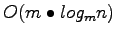
Batch filtering is used to represent a data structure of size $N$ in such a way that $K$ constant size output queries can be answered in $O((n+k) log_{m}n$ I/Os. This is accomplished by representing the data structure as a directed acyclical graph (DAG) isomorphic to the original data structure and filtering the K queries down through this structure.

Time Forward Processing

In [9] the Time Forward Processing technique is presented as a technique for solving circuit like and similar problems in external memory. The original problem was specified for bounded in degree boolean circuits, see Fig. 1, which is a directed acyclic graph, dag, where vertices having an in-degree of at most $\frac{M}{2}$ . The entire structure is stored in external memory.

Node labels come from a total order such that for every edge $(v,w)$ node $v$ occurs before $w$ . The time forward processing works by processing each vertex at time $v$ , with the trick being to ensure that all inputs for node $v$ are available in main memory at time $v$ . Time foward processing techniques were developed by [9] who used bucketing to build a tree of time intervals and later in [3] where an external memory priority queue based on the buffer-tree is presented which provides an alternative implementation for time-forward processing.

Figure 1: A bounded fan-in circuit.

External Memory Priority Queue

An alternate implementation of time forward processing is proposed by [3] where an external priority queue based based on the buffer-tree is proposed as a simpler alternative to the bucketing technique in [9]. In addition to the somewhat complex nature of the bucketing technique the technique can only be employed with large values of m such that 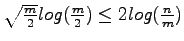$\sqrt{\frac{m}{2}} log(\frac{m}{2}) \leq 2 log(\frac{n}{m})$ . While this later restriction is not a major hurdle, as this condition holds for most modern computer systems, it is removed by the simpler external priority queue technique.

A search tree can be used to implement a priority queue because the smallest element will be stored in the leftmost leaf and as such the Deletemin operation can be easily implemented by deleting this leaf. The buffer-tree maintains buffers associated with each non-leaf node. When an item is inserted (or deleted) rather than be filtered down through the tree to the approriate leaf the item is stored in the buffer of the root node. When a buffer becomes full the items it contains are then distributed among the buffers of its children and so on down to the leaves. The use of buffers creates one problem for the buffer tree as a priority queue that being that the smallest item may not be stored in the leftmost leaf, but may be stored in a buffer on the path between the root and this leaf.

To enable the buffer-tree as an external memory priority queue the following alteration was made to its operation. When a Deletemin operation was performed the buffers along a path from the root to the leftmost leaf are flushed with $O(m \bullet log_{m}n)$ I/Os. Following this operation the we are ensure that the $\frac{1}{4}m\bullet B$ Deletemin operations can be performed without any further I/Os if we delete the $\frac{1}{4}m\bullet B$ smallest elements and keep them in internal memory. Storing these elements in internal memory necessitates checking insertions and deletions against this minimal element buffer but doing so is a simple proceedure. The total cost of an arbitrary sequences of insertions, deletions, and deletemin operations on an initially empty buffer tree is $O(n log_{m}n)$ I/Os, with an amortized per-operation cost of $O(\frac{log_{m}n}{B})$ .

This efficient external memory priority queue makes the implementation of time forward processing quite straightforward. When a node is evaluated the outputs from that node are inserted into the priority queue with the labels of the receiving nodes as their priority. As elements are processed in sorted order we can always access the inputs for the next node by performing the proper number of deletemin operations on the priority queue. The I/O bound of $O(n log_{m}n)$ is achieved as this is the bound associated with the priority queue.