Logic
-
Logic gives precise meaning to statements
- tells us precisely what statements mean
- allows computers to reason without the baggage of language
-
the building block of logic is the proposition
-
a declarative sentence that is either true or false
- "Carleton University is located in Ottawa"
- "$1+1=2$"
- "$1+1=3$"
-
a declarative sentence that is either true or false
-
sentences that are not declarative are not propositions:
- "How are you feeling today?"
- "Pay attention!"
-
sentences that are neither true nor false are not propositions:
- "$x+y=z$"
- "This sentence is false."
- we can assign propositions names like $a,b,c,\ldots$ for short
- the truth value of a proposition is either $T$ (true) or $F$ (false)
- a single proposition should express a single fact:
- "It is Monday and I am in class" is better expressed as two propositions: "It is Monday", "I am in class"
Connectives
How do we assert two propositions are true (or otherwise related) at once?- use connectives to create compound propositions
-
negation: if $p$ is a propostion, then "it is not the case that $p$ is true" is a compound proposition called the negation of $p$, written $\neg p$
- The negation of "The network is functioning normally" is "It is not the case that the network is functioning normally" (or just "The network is not functioning normally")
- as a general rule, the original propositions you define should not contain a negation
- the truth value of a negation can be determined using a truth table: \begin{array}{c|c} p & \neg p \\\hline T & F \\ F & T \\ \end{array}
-
conjunction ("and"): if $p$ and $q$ are propositions, then "$p$ and $q$" is a compound proposition called the conjunction of $p$ and $q$, written $p \wedge q$
- "The program is fast and the program is accurate" (or just, "The program is fast and accurate")
- conjunction has the following truth table: \begin{array}{cc|c} p & q & p \wedge q \\\hline T & T & T \\ T & F & F \\ F & T & F \\ F & F & F\\ \end{array}
- there are many ways to express conjunction: "and", "but", "so", "also", ...
-
disjunction ("or"): if $p$ and $q$ are propositions, then "$p$ or $q$" is a compound proposition called the disjunction of $p$ and $q$, written $p \vee q$
- "I work hard or I fail"
- disjunction has the following truth table: \begin{array}{cc|c} p & q & p \vee q \\\hline T & T & T \\ T & F & T \\ F & T & T \\ F & F & F \\ \end{array}
- disjunction in logic differs a bit from casual language
-
there are two kinds of "or": inclusive and exclusive
- inclusive: "Students must have taken computer science or calculus to enroll in this course"
- exclusive: "The meal comes with a soup or salad"
- we will always assume inclusive or when we use the $\vee$ symbol
- for exclusive or, we write $\oplus$ and use the following truth table: \begin{array}{cc|c} p & q & p \oplus q \\\hline T & T & F \\ T & F & T \\ F & T & T \\ F & F & F \\ \end{array}
-
implication ("if...then"): if $p$ and $q$ are propositions, then the implication "if $p$ then $q$" is a compound propositon, written $p \rightarrow q$
- "If the website is down, then the technical support person must fix it"
- We call $p$ the hypothesis and $q$ the conclusion
- implication has the following truth table: \begin{array}{cc|c} p & q & p \rightarrow q \\\hline T & T & T \\ T & F & F \\ F & T & T \\ F & F & T \\ \end{array}
-
there are many ways to write $p \rightarrow q$ in English:
- if $p$ then $q$
- $p$ implies $q$
- if $p$, $q$
- $p$ only if $q$
- $p$ is sufficient for $q$
- a sufficient condition for $q$ is $p$
- $q$ if $p$
- $q$ whenever $p$
- $q$ when $p$
- $q$ is necessary for $p$
- $q$ follows from $p$
- a necessary condition for $p$ is $q$
- when $p$ is false, $p \rightarrow q$ is true regardless of the truth value of $q$
-
given $p \rightarrow q$, we can define a few special propositions:
- $q \rightarrow p$ is the converse
- $\neg q \rightarrow \neg p$ is the contrapositive
- $\neg p \rightarrow \neg q$ is the inverse
-
biconditional ("if and only if"): if $p$ and $q$ are propositions, then the biconditional "$p$ if and only if $q$" is a compound propositon, written $p \leftrightarrow q$
- "You will pass this course if and only if you study"
- The biconditional has the following truth table: \begin{array}{cc|c} p & q & p \leftrightarrow q \\\hline T & T & T \\ T & F & F \\ F & T & F \\ F & F & T \\ \end{array}
- "if and only if" is often abbreviated to "iff"
- we say "$p$ is necessary and sufficient for $q$", "if $p$ then $q$, and conversely", or "$p$ iff $q$"
- we will use brackets as much as possible to make precedence clear
-
as a general rule, negation applies to whatever is directly after only
- $\neg p \vee q$ is $(\neg p) \vee (q)$
- use brackets for everything else so there is no ambiguity
Translating Sentences
-
Let $a$ be the proposition "the computer lab uses Linux", $b$ be the proposition "a hacker breaks into the computer" and $c$ be the proposition "the data on the computer is lost."
- $(a \rightarrow \neg b) \wedge (\neg b \rightarrow \neg c)$ means "If the computer in the lab uses Linux then a hacker will not break into the computer, and if a hacker does not break into the computer then the data on the computer will not be lost."
- $\neg(a \vee \neg b)$ means "It is not the case that either the computer in the lab uses Linux or a hacker will break into the computer." (This is a bit awkward. We will learn how to phrase this better later.)
- $c \leftrightarrow (\neg a \wedge b)$ means "The data on the computer is lost if and only if the computer in the lab does not use Linux and a hacker breaks into the computer."
-
How could we translate "If the hard drive crashes then the data is lost"?
- Let $h$ be the proposition "the hard drive crashes" and $d$ be the proposition "the data is lost." The sentence translates to $h \rightarrow d$.
-
How could we translate "The infrared scanner detects motion only if the intruder is in the room or the scanner is defective"?
- Let $m$ be the proposition "the infrared scanner detects motion", $i$ be the proposition "the intruder is in the room" and $d$ be the proposition "the scanner is defective." The sentence translates to $m \rightarrow (i \vee d)$.
-
How could we translate "If the server is down and the network connection is lost, then email is not available but I can still play games" into propositional logic?
- Let $s$ be the proposition "the server is down", $n$ be the proposition "the network connection is lost", $e$ be the proposition "email is available" and $g$ be the proposition "I can play games." The sentence translates to $(s \wedge n) \rightarrow (\neg e \wedge g)$.
Truth Tables
How can we determine the truth value of compound propositions?- we need the truth values of the propositions that make them up
- we can use truth tables to look at all possible combinations
- one column for every proposition
- break the compound proposition into parts
- one row for every truth value combination
- fill the table in by working with smaller parts first and building to the whole compound proposition
- $((a \vee b) \wedge (\neg a \vee c)) \rightarrow (b \vee c)$ \begin{array}{ccc|ccccc|c} a & b & c & a \vee b & \neg a & \neg a \vee c & (a \vee b) \wedge (\neg a \vee c) & b \vee c & ((a \vee b) \wedge (\neg a \vee c)) \rightarrow (b \vee c)\\\hline T & T & T & T & F & T & T & T & T \\ T & T & F & T & F & F & F & T & T \\ T & F & T & T & F & T & T & T & T \\ T & F & F & T & F & F & F & F & T \\ F & T & T & T & T & T & T & T & T \\ F & T & F & T & T & T & T & T & T \\ F & F & T & F & T & T & F & T & T \\ F & F & F & F & T & T & F & F & T \\ \end{array} Observe that every row in the last column has value $T$. Therefore, the proposition is a tautology.
- $\neg ((\neg a \rightarrow (\neg b \vee c)) \leftrightarrow (b \rightarrow (a \vee c)))$ \begin{array}{ccc|ccccccc|c} a & b & c & \neg a & \neg b & \neg b \vee c & \overbrace{\neg a \rightarrow (\neg b \vee c)}^X & a \vee c & \overbrace{b \rightarrow (a \vee c)}^Y & X \leftrightarrow Y & \neg (X \leftrightarrow Y) \\\hline T & T & T & F & F & T & T & T & T & T & F \\ T & T & F & F & F & F & T & T & T & T & F \\ T & F & T & F & T & T & T & T & T & T & F \\ T & F & F & F & T & T & T & T & T & T & F \\ F & T & T & T & F & T & T & T & T & T & F \\ F & T & F & T & F & F & F & F & F & T & F \\ F & F & T & T & T & T & T & T & T & T & F \\ F & F & F & T & T & T & T & F & T & T & F \\ \end{array} Observe that every row in the last column has value $F$. Therefore, the proposition is a contradiction. Notice how we relabelled two large compound propositions in order to save space in the truth table.
- $\neg(a \wedge b) \leftrightarrow ((a \vee b) \wedge \neg(a \vee \neg b))$ \begin{array}{cc|ccccccc|c} a & b & a \wedge b & \overbrace{\neg(a \wedge b)}^X & a \vee b & \neg b & a \vee \neg b & \neg(a \vee \neg b) & \overbrace{(a \vee b) \wedge \neg(a \vee \neg b)}^Y & X \leftrightarrow Y \\\hline T & T & T & F & T & F & T & F & F & F \\ T & F & F & T & T & T & T & F & F & T \\ F & T & F & T & T & F & F & T & T & T \\ F & F & F & T & F & T & T & F & F & T \\ \end{array} Observe that the rows of the last column have both $T$s and $F$s. Therefore, the proposition is a contingency.
Logical Equivalences
There is often more than one way to write a proposition. For instance, $p$ and $\neg \neg p$ mean the same thing. We write $p \equiv \neg \neg p$ to mean "the proposition $p$ is logically equivalent to the proposition $\neg \neg p$". How do we tell if two expressions are logically equivalent? The first method is to use truth tables:- logical equivalence = same truth tables
- to see if two expressions are logically equivalent, just check their truth tables to see if they match
- To check if $\neg (p \vee q)$ and $\neg p \wedge \neg q$ are logically equivalent: \begin{array}{cc|ccccc} p & q & p \vee q & \neg (p \vee q) & \neg p & \neg q & \neg p \wedge \neg q \\\hline T & T & T & F & F & F & F \\ T & F & T & F & F & T & F \\ F & T & T & F & T & F & F \\ F & F & F & T & T & T & T \\ \end{array} Since columns corresponding to $\neg (p \vee q)$ and $(\neg p \wedge \neg q)$ match, the propositions are logically equivalent. This particular equivalence is known as De Morgan's Law.
- Are $p \vee (q \wedge r)$ and $(p \vee q) \wedge (p \vee r)$ logically equivalent? \begin{array}{ccc|ccccc} p & q & r & q \wedge r & p \vee (q \wedge r) & p \vee q & p \vee r & (p \vee q) \wedge (p \vee r) \\\hline T & T & T & T & T & T & T & T \\ T & T & F & F & T & T & T & T \\ T & F & T & F & T & T & T & T \\ T & F & F & F & T & T & T & T \\ F & T & T & T & T & T & T & T \\ F & T & F & F & F & T & F & F \\ F & F & T & F & F & F & T & F \\ F & F & F & F & F & F & F & F \\ \end{array} Since columns corresponding to $p \vee (q \wedge r)$ and $(p \vee q) \wedge (p \vee r)$ match, the propositions are logically equivalent. This particular equivalence is known as the Distributive Law.
- Identity Law: $p \wedge T \equiv p$ and $p \vee F \equiv p$
- Idempotent Law: $p \vee p \equiv p$ and $p \wedge p \equiv p$
- Domination Law: $p \vee T \equiv T$ and $p \wedge F \equiv F$
- Negation Law: $p \vee \neg p \equiv T$ and $p \wedge \neg p \equiv F$
- Double Negation Law: $\neg(\neg p) \equiv p$
- Commutative Law: $p \vee q \equiv q \vee p$ and $p \wedge q \equiv q \wedge p$
- Associative Law: $(p \vee q) \vee r \equiv p \vee (q \vee r)$ and $(p \wedge q) \wedge r \equiv p \wedge (q \wedge r)$
- Distributive Law: $p \vee (q \wedge r) \equiv (p \vee q) \wedge (p \vee r)$ and $p \wedge (q \vee r) \equiv (p \wedge q) \vee (p \wedge r)$
- Absorption Law: $p \vee (p \wedge q) \equiv p$ and $p \wedge (p \vee q) \equiv p$
- De Morgan's Law: $\neg(p \wedge q) \equiv \neg p \vee \neg q$ and $\neg(p \vee q) \equiv \neg p \wedge \neg q$
- Implication Equivalence: $p \rightarrow q \equiv \neg p \vee q$
- Biconditional Equivalence: $p \leftrightarrow q \equiv (p \rightarrow q) \wedge (q \rightarrow p)$
- $\neg(p \vee (\neg p \wedge q))$ and $\neg p \wedge \neg q$ \begin{array}{llll} \neg(p \vee (\neg p \wedge q)) & \equiv & \neg p \wedge \neg(\neg p \wedge q)) & \text{De Morgan's Law} \\ & \equiv & \neg p \wedge (\neg\neg p \vee \neg q)) & \text{De Morgan's Law} \\ & \equiv & \neg p \wedge (p \vee \neg q)) & \text{Double Negation Law} \\ & \equiv & (\neg p \wedge p) \vee (\neg p \wedge q)) & \text{Distributive Law} \\ & \equiv & F \vee (\neg p \wedge q)) & \text{Negation Law} \\ & \equiv & \neg p \wedge \neg q & \text{Identity Law} \\ \end{array} Since each proposition is logically equivalent to the next, we must have that $\neg(p \vee (\neg p \wedge q))$ and $\neg p \wedge \neg q$ are logically equivalent.
- Is $(p \wedge q) \rightarrow (p \vee q)$ a tautology, contradiction or contingency? \begin{array}{llll} (p \wedge q) \rightarrow (p \vee q) & \equiv & \neg(p \wedge q) \vee (p \vee q) & \text{Implication Equivalence} \\ & \equiv & (\neg p \vee \neg q) \vee (p \vee q) & \text{De Morgan's Law} \\ & \equiv & (\neg p \vee p) \vee (q \vee \neg q) & \text{Associative and Commutative Laws} \\ & \equiv & T \vee T & \text{Negation Law} \\ & \equiv & T & \text{Domination Law} \\ \end{array} Since each proposition is logically equivalent to the next, we must have that $(p \wedge q) \rightarrow (p \vee q)$ and $T$ are logically equivalent. Therefore, regardless of the truth values of $p$ and $q$, the truth value of $(p \wedge q) \rightarrow (p \vee q)$ is $T$. Thus, $(p \wedge q) \rightarrow (p \vee q)$ is a tautology.
- $\neg p \vee \neg q$ and $p \wedge q$ \begin{array}{llll} \neg p \vee \neg q & \equiv & \neg(p \wedge q) & \text{De Morgan's Law} \\ \end{array} However, $p \wedge q$ is not equivalent to $\neg(p \wedge q)$, since it is its negation. Therefore, the two propositions are not logically equivalent.
- $(p \rightarrow q) \rightarrow r)$ and $p \rightarrow (q \rightarrow r)$ \begin{array}{ccc|cccc} p & q & r & p \rightarrow q & q \rightarrow r & (p \rightarrow q) \rightarrow r & p \rightarrow (q \rightarrow r) \\\hline T & T & T & T & T & T & T \\ T & T & F & T & F & F & F \\ T & F & T & F & T & T & T \\ T & F & F & F & T & T & T \\ F & T & T & T & T & T & T \\ F & T & F & T & F & F & T \\ F & F & T & T & T & T & T \\ F & F & F & T & T & F & T \\ \end{array} Since the last two columns do not match, the propositions are not logically equivalent.
- $\neg p \rightarrow (q \rightarrow r)$ and $q \rightarrow (p \vee r)$ \begin{array}{ccc|ccccc} p & q & r & \neg p & q \rightarrow r & p \vee r & \neg p \rightarrow (q \rightarrow r) & q \rightarrow (p \vee r) \\\hline T & T & T & F & T & T & T & T \\ T & T & F & F & F & T & T & T \\ T & F & T & F & T & T & T & T \\ T & F & F & F & T & T & T & T \\ F & T & T & T & T & T & T & T \\ F & T & F & T & F & F & F & F \\ F & F & T & T & T & T & T & T \\ F & F & F & T & T & F & T & T \\ \end{array} Since the last two columns match, the propositions are logically equivalent. We can also see this using logical equivalences: \begin{array}{llll} \neg p \rightarrow (q \rightarrow r) & \equiv & \neg \neg p \vee (q \rightarrow r) & \text{Implication Equivalence} \\ & \equiv & p \vee (q \rightarrow r) & \text{Double Negation Law} \\ & \equiv & p \vee (\neg q \vee r) & \text{Implication Equivalence} \\ & \equiv & \neg q \vee (p \vee r) & \text{Associative and Commutative Laws} \\ & \equiv & q \rightarrow (p \vee r) & \text{Implication Equivalence} \\ \end{array} Since each proposition is logically equivalent to the next, we must have that the two propositions are logically equivalent.
- Are the statements "if food is good, it is not cheap" and "if food is cheap, it is not good" saying the same thing? Let $g$ be the proposition "food is good" and $c$ be the proposition "food is cheap." The first statement is $g \rightarrow \neg c$ and the second statement is $c \rightarrow \neg g$. We now apply some logical equivalences. \begin{array}{llll} g \rightarrow \neg c & \equiv & \neg g \vee \neg c & \text{Implication Equivalence} \\ & \equiv & \neg c \vee \neg g & \text{Commutative Law} \\ & \equiv & c \rightarrow \neg g & \text{Implication Equivalence} \\ \end{array} Since the two statements are logically equivalent, they are saying the same thing.
Predicate Logic
Problem with propositional logic: how does one say, "Everyone in this class is a student"?- not very useful to use that as a proposition: it says too much!
- propositions should talk about one thing: "person $X$ is in this class", "person $X$ is a student"
- so we could say "$X_1$ is in this class $\wedge$ $X_1$ is a student $\wedge$ $X_2$ is in this class $\wedge$ $X_2$ is a student $\wedge \cdots$"
- two propositions per person: this is a lot of work!
Idea: "being a student" and "being in this class" are properties that people can have, and "everyone" quantifies which people have the property. We can define a propositional function that asserts that a predicate is true about some object.
Suppose $S$ denotes the predicate "is a student". Then $S(x)$ means "$x$ is a student" for some object $x$. This works for all predicates: "is greater than", "is shorter than", "is a boat", $\ldots$
Once we have defined a propositional function, any object we give to it produces a truth value. For example, if $P(x)$ means "$x$ is greater than $3$", then:
- $P(2)$ is false
- $P(3)$ is false
- $P(4)$ is true
- $P(1,2)$ is false
- $P(2,1)$ is true
Universe of Discourse
Before we can think about quantifiers, we need to think about the universe of discourse. In the above example about students, there are at least two possible universes of discourse. If the universe is "all people in the class", then saying $x_1$ is in this class" is redundant. However, if the universe of discourse is "all people", then it is important!
As another example, consider $P(x)$ to denote "$x$ is greater than $3$". Here, the universe is assumed to be, say, the set of all real numbers. If the universe of discourse was the set of all people, we would have statements like "John is greater than $3$", which makes no sense.
It is important to define a universe of discourse! Think of the universe of discourse as the set of all values (names) that you can plug into the propositional functions being considered.
Universal Quantification
Given a propositional function $P(x)$, the \emph{universal quantification} of $P(x)$ is the proposition "$P(x)$ is true for all values $x$ in the universe of discourse." We write $\forall x\; {P(x)}$ and say "for all $x$, $P(x)$" or "for every $x$, $P(x)$." The symbol $\forall$ is the universal quantifier.
This notation is essentially shorthand. If the universe of discourse consists of the objects $x_1,x_2,\ldots$, then $\forall x\;{P(x)}$ means $P(x_1) \wedge P(x_2) \wedge \cdots$. Of course, if the universe of discourse is infinite (for example, the integers or real numbers), then such shorthand becomes necessary.
Observe that since $\forall x\;{P(x)}$ is essentially a conjunction, it must be the case that it has truth value $T$ precisely when the predicate is true for all objects in the universe of discourse and $F$ otherwise. Therefore, if the predicate $P$ is false for at least one object in the universe of discourse, then $\forall x\;{P(x)}$ has truth value $F$. Here are some examples that use universal quantification:
- Let $P(x)$ denote "$x$ is greater than $5$", where the universe of discourse is the set of integers. Then the truth value of $\forall x\;{P(x)}$ is $F$, since, for example, $P(4)$ is $F$. Note that if the universe of discourse had been the set of all integers greater than or equal to $6$, then $\forall x \;{P(x)}$ would have truth value $T$.
- Let $P(x)$ denote "$x^2 \ge x$" where the universe of discourse is the set of real numbers. Is $\forall x\;{P(x)}$ true? What if the universe of discourse is the set of integers? Observe that $x^2 \ge x$ if and only if $x^2 - x \ge 0$, which is true if and only if $x(x-1) \ge 0$, which is true if and only if $x \le 0$ or $x \ge 1$. Therefore, if the universe of discourse is the set of real numbers, any real number strictly between $0$ and $1$ gives an example where the statement is false. For example, $(1/2)^2 = 1/4 \lt 1/2$. Therefore, $\forall x\;{P(x)}$ is false if the universe of discourse is the set of real numbers.If the universe of discourse is the set of integers, however, $\forall x\;{P(x)}$ is true, since there is no integer strictly between $0$ and $1$.
Exisential Quantification
Given a propositional function $P(x)$, the existential quantification of $P(x)$ is the proposition "$P(x)$ is true for at least one value $x$ in the universe of discourse." We write $\exists x\;{P(x)}$ and say "there exists an $x$ such that $P(x)$" or "for some $x$, $P(x)$." The symbol $\exists$ is the existential quantifier.
Again, this notation is essentially shorthand. If the universe of discourse consists of the objects $x_1,x_2,\ldots$, then $\exists x \;{P(x)}$ means $P(x_1) \vee P(x_2) \vee \cdots$.
Observe that since $\exists x\;{P(x)}$ is essentially a disjunction, it must be the case that it has truth value $T$ precisely when the predicate is true for at least one object in the universe of discourse and $F$ otherwise. Therefore, if the predicate $P$ is false for all objects in the universe of discourse, then $\exists x\;{P(x)}$ has truth value $F$. Here are some examples that use existential quantification:
- Let $P(x)$ denote "$x$ is greater than $5$", where the universe of discourse is the set of integers. Then the proposition $\exists x\;{P(x)}$ has truth value $T$, since, for example, $P(6)$ is true. If the universe of discourse had been the set of all integers less than or equal to $5$, then $\exists x\;{P(x)}$ would have truth value $F$.
- Let $P(x)$ denote "$x = x + 1$", where the universe of discourse is the set of integers. Then the truth value of $\exists x\;{P(x)}$ is $F$, because no integer has this property (since it implies that $0 = 1$).
Binding of Quantifiers
The scope of a quantifier is the smallest proposition following it: $$ \underbrace{\exists x\;{P(x)}}_{\text{$x$ applies here}} \wedge \underbrace{Q(x)}_{\text{but $x$ has no meaning here}} $$ We would instead write $\exists x\;{(P(x) \wedge Q(x))}$.
It is valid to write, for example, $\exists x\;{P(x)} \wedge \exists x\;{Q(x)}$, but the $x$ in each quantifier could be completely different elements of the universe of discourse! Conversely, we might want to make sure they are not the same: $\exists x \;{\exists y\;{(P(x) \wedge Q(y) \wedge (x \neq y))}}$.
For example, if the universe of discourse is the set of integers, $E(x)$ means "$x$ is a even", and $O(x)$ means "$x$ can odd":
- $\exists x\;{E(x)}$ is true, since (for example) $4$ is an even integer
- $\exists x\;{O(x)}$ is true, since (for example) $3$ is an odd integer
- $\exists x\;{E(x)} \wedge \exists x\;{O(x)}$ is true, since the $x$s can be different
- $\exists x\;{(E(x) \wedge O(x))}$ is false, since no integer is both even and odd
Negating Quantifiers
How do we negate a quantified statement?- What is the negation of "all people like math"?
- "it is not the case that all people like math"
- $\equiv$ true when at least one person does not like math
- $\equiv$ there exists one person who does not like math
- What is the negation of "at least one person likes math"?
- "it is not the case that at least one person likes math"
- $\equiv$ true when there are no people who like math
- $\equiv$ every person does not like math
We have the following quantifier negation rules:
- $\neg \forall x\;{P(x)} \equiv \exists x\;{\neg P(x)}$
- $\neg \exists x\;{P(x)} \equiv \forall x\;{\neg P(x)}$
- The negation of $\forall x\;{(x^2 > x)}$ is $\neg \forall x\;{(x^2 > x)} \equiv \exists x\;{\neg(x^2 > x)} \equiv \exists x\;{(x^2 \le x)}$
- Then negation of $\exists x\;{(x^2 = 2)}$ is $\neg \exists x\;{(x^2 = 2)} \equiv \forall x\;{\neg(x^2 = 2)} \equiv \forall x\;{(x^2 \neq 2)}$
Translating Sentences with Predicates and Quantifiers
- Universal quantifiers: look for keywords like "every", "all"
- Existential quantifiers: look for keywords like "some", "at least one"
- "Every student in this class will learn about logic"
- Let $S(x)$ denote "$x$ is a student in this class" and $L(x)$ denote "$x$ will learn about logic".
- The sentence is $\forall x\;{(S(x) \rightarrow L(x))}$.
- Note: the answer is not $\forall x\;{S(x)} \rightarrow L(x)$ because the $x$ in $L(x)$ is not bound.
- Note: the answer is not $\forall x\;{(S(x) \wedge L(x))}$ because this is saying every person is a student in this class and will learn about logic (too strong!)
- "Some student in this class will learn about calculus"
- Let $S(x)$ denote "$x$ is a student in this class" and $C(x)$ denote "$x$ will learn about calculus".
- The sentence is $\exists x\;{(S(x) \wedge C(x))}$.
- Note: the answer is not $\exists x\;{S(x)} \wedge L(x)$ because the $x$ in $C(x)$ is not bound.
- Note: the answer is not $\exists x\;{(S(x) \rightarrow C(x))}$ because this does not assert the existence of any students in this class (too weak!)
- Let $I(x)$ denote "$x$ is an instructor" and $K(x)$ denote "$x$ knows everything." Then the statement "no instructor knows everything" can be translated as $\neg \exists x\;{(I(x) \wedge K(x))}$.
- We can apply quantifier negation to this to get $\forall x\;{\neg(I(x) \wedge K(x))}$.
- Applying De Morgan's Law, we get $\forall x\;{(\neg I(x) \vee \neg K(x))}$.
- Applying Implication Equivalence, we get $\forall x\;{(I(x) \rightarrow \neg K(x))}$ ("if you are an instructor, then you don't know everything").
- The statement "some instructors don't know everything" can be translated as $\exists x\;{(I(x) \wedge \neg K(x))}$.
- Let $F(x,y)$ denote "$x$ and $y$ are friends." Then $\forall a\;{\exists b\;{F(a,b)}}$ means "everyone has at least one friend." Note that this is not the same as $\exists b\;{\forall a\;{F(a,b)}}$, since this means "there is one person who is friends with everyone."
- Let $M(x)$ denote "$x$ is male", $F(x)$ denote "$x$ is female", $L(x)$ denote "$x$ is a student in this class" and $K(x,y)$ denote "$x$ knows $y$." Then the statement "every female student in this class knows at least one male student in this class" can be translated as $\forall x\;{((F(x) \wedge L(x)) \rightarrow \exists y\;{(M(y) \wedge L(y) \wedge K(x,y))})}$.
- Let the universe of discourse be all Olympic athletes. Let $D(x)$ denote "$x$ uses performance enhancing drugs" and $M(x)$ denote "$x$ wins a medal." The direct translation of $\neg \forall x\;{(\neg M(x) \rightarrow \neg D(x))}$ is awkward. Applying some logical equivalences, we get \begin{array}{llll} \neg \forall x\;{(\neg M(x) \rightarrow \neg D(x))}$ & \equiv & \exists x\;{\neg(\neg M(x) \rightarrow \neg D(x))} & \text{Quantifier Negation} \\ & \equiv & \exists x\;{\neg(\neg \neg M(x) \vee \neg D(x))} & \text{Implication Equivalence} \\ & \equiv & \exists x\;{(\neg \neg \neg M(x) \wedge \neg \neg D(x))} & \text{De Morgan's Law} \\ & \equiv & \exists x\;{(\neg M(x) \wedge D(x))} & \text{Double Negation Law} \\ \end{array} This translates much more cleanly to "there is at least one olympic athlete who uses performance enhancing drugs but does not win a medal."
- Let the universe of discourse be all people. Let $F(x)$ denote "$x$ is female", $P(x)$ denote "$x$ is a parent" and $M(x,y)$ denote "$x$ is the mother of $y$." Then the statement "if a person is female and a parent, then that person is someone's mother" can be translated as $\forall x\;{((F(x) \wedge P(x)) \rightarrow \exists y\;{M(x,y)})}$, or equivalently, $\forall x\;{\exists y\;{((F(x) \wedge P(x)) \rightarrow M(x,y))}}$.
- Let the universe of discourse be all people and let $B(x,y)$ denote "$y$ is the best friend of $x$." To translate the statement "everyone has exactly one best friend", note that to have exactly one best friend, say $y$, then no other person $z$ is that person's best friend, unless $y = z$. The statement can therefore be translated as $\forall x\;{\exists y\;{(B(x,y) \wedge \forall z\;{((z \neq y) \rightarrow \neg B(x,z)))}}}$.
Arguments and Validity
Now that we know how to state things precisely, we are ready to think about putting statements together to form arguments. A rigorous argument that is valid constitutes a proof. We need to put the statements together using valid rules.For example, given the premises:
- "if it is cloudy outside, then it will rain"
- "it is cloudy outside"
a conclusion might be "it will rain". Intuitively, this seems valid.
An argument is valid if the truth of the premises implies the conclusion. Given premises $p_1, p_2, \ldots, p_n$, and conclusion $c$, the argument is valid if and only if $(p_1 \wedge p_2 \wedge \cdots \wedge p_n) \rightarrow c$. Note that false premises can lead to a false conclusion!Rules of Inference
How do we show validity? We use the rules of inference:- Addition: given $p$, conclude $p \vee q$
- Conjunction: given $p$ and $q$, conclude $p \wedge q$
- Simplification: given $p \wedge q$, conclude $p$ and $q$
- Modus Ponens: given $p$ and $p \rightarrow q$, conclude $q$
- Modus Tollens: given $\neg q$ and $p \rightarrow q$, conclude $\neg p$
- Hypothetical Syllogism: given $p \rightarrow q$ and $q \rightarrow r$, conclude $p \rightarrow r$
- Disjunctive Syllogism: given $p \vee q$ and $\neg p$, conclude $q$
- Resolution: given $p \vee q$ and $\neg p \vee r$, conclude $q \vee r$
- Consider the argument:
- It is not sunny this afternoon and it is colder than yesterday.
- We will go swimming only if it is sunny.
- If we do not go swimming, then we will take a canoe trip.
- If we take a canoe trip, we will be home by sunset.
- Therefore, we will be home by sunset.
- Consider the argument:
- If you send me an email message, then I will finish writing the program.
- If you do not send me an email message, then I will go to sleep early.
- If I go to sleep eaerly, then I will wake up feeling refreshed.
- Therefore, if I do not finish writing the program, I will wake up feeling refreshed.
- Consider the arugment:
- Either I study or I fail.
- I did not study.
- Therefore, I fail.
Not all arguments are valid! To show an argument is invalid, find truth values for each proposition that make all of the premises true, but the conclusion false.
This works because proving an argument is valid is just showing that an implication is true. Therefore, to show an argument is invalid, we need to show that the implication is false. An implication is false only when the hypothesis is true and the conclusion is false. Since the hypothesis is the conjunction of the premises, this means that each premise is true and the conclusion is false. $$ \underbrace{(p_1 \wedge p_2 \wedge \cdots \wedge p_n)}_{\text{all $T$}} \rightarrow \underbrace{c}_{F} $$
- Consider the argument:
- If I did all the suggested exercises, then I got an A+
- I got an A+
- Therefore, I did all of the suggested exercises.
Arguments with Quantified Statements
Until now, we have restricted our attention to propositional logic. Recall that $P(x)$ is a propositional function, and so when $x$ is an element of the universe of discourse, we simply have a proposition that can be dealt with using the rules of inference for propositions. For predicate logic, we need a few more rules of inference that will allow us to deal with quantified statements.- Universal Instantiation: given $\forall x\;{P(x)}$, conclude $P(c)$ for any $c$ in the universe of discourse (if $P$ holds for everything, it must hold for each particular thing)
- Existential Generalization: given $P(c)$ for some $c$ in the universe of discourse, conclude $\exists x\;{P(x)}$ (if I can find an element for which $P$ is true, then there must exist at least one such element)
- Universal Generalization: given $P(c)$ for an arbitrary $c$ in the universe of discourse, conclude $\forall x {P(x)}$ (here, $c$ must be arbitrary; it must hold for any $c$!)
- Existential Instantiation: given $\exists x\;{P(x)}$, conclude $P(c)$ for some $c$ in the universe of discourse (you must pick a new $c$ about which you know nothing else)
- Consider the following argument, where the universe of discourse is the set of all things.:
- All men are mortal.
- Socrates is a man.
- Therefore, Socrates is mortal.
- Consider the following argument, where the universe of discourse is the set of all people.
- A student in this class has not read the textbook.
- Everyone in this class did well on the first assignment.
- Therefore, someone who did well on the first assignment has not read the textbook.
- Consider the following argument, where the universe of discourse is the set of people.
- All human beings are from Earth.
- Every person is a human being.
- Therefore, every person is from Earth
- Consider the following argument, where the universe of discourse is the set of people.
- If John knows discrete mathematics, he will pass this course.
- John knows discrete mathematics.
- Therefore, everyone will pass this course
Methods of proof
How do we go about forming arguments (proofs)?- Direct proofs: to prove an implication $p \rightarrow q$, start by assuming that $p$ is true, and then prove that $q$ is true under this assumption.
-
Prove that if $n$ is an odd integer, then $n^2$ is an odd integer.
Assume that $n$ is an odd integer. Therefore, we can write $n=2k+1$ for some integer $k$. So $n^2 = (2k+1)^2 = 4k^2 + 4k + 1 = 2(2k^2 + 2k) + 1$. This has form $2k'+1$ for an integer $k'$ and is therefore odd.
-
Prove that if $n$ is an odd integer, then $n^2$ is an odd integer.
- Indirect proof: Recall that $p \rightarrow q \equiv \neg q \rightarrow \neg p$. Therefore, to prove $p \rightarrow q$, we could instead prove $\neg q \rightarrow \neg p$ using a direct proof: assume $\neg q$ and prove $\neg p$.
-
Prove that if $3n + 2$ is odd, then $n$ is odd.
We instead prove that if $n$ is even, then $3n + 2$ is even. Assume $n$ is even; then $n = 2k$ for some integer $k$. So $3n + 2 = 3(2k) + 2 = 6k + 2 = 2(3k + 1)$, which has the form $2k'$ for an integer $k'$ and is therefore even.
-
Prove that the sum of two rational numbers is rational.
We will attempt to prove this directly: if $r$ and $s$ are rational numbers, then $r + s$ is a rational number. Assume that $r$ and $s$ are rational numbers. Then $r = a/b$ and $s = c/d$ where $a,b,c,d \in \mathbb{Z}$ and $b,d \neq 0$ by the definition of rational numbers. Now, $r + s = (ad + bc)/bd$. Since $a,b,c,d \in \mathbb{Z}$, $ad + bc$ and $bd$ are both integers. Since $b,d \neq 0$, we have $bd \neq 0$. Therefore, $r + s$ is rational. A direct proof succeeded!
-
Prove that if $n$ is an integer and $n^2$ is odd, then $n$ is odd.
We will attempt to prove this directly. Assume $n$ is an integer and $n^2$ is odd. Then $n^2 = 2k + 1$ and so $n = \pm\sqrt{2k + 1}$. It is not obvious how to proceed at this point, so we will turn to an indirect proof. Assume $n$ is even. Then $n = 2k$, and so $n^2 = (2k)^2 = 4k^2 = 2(2k^2)$. Therefore, $n^2$ is even. An indirect proof worked!
-
Prove that if $3n + 2$ is odd, then $n$ is odd.
- Vacuous/trivial proofs: When trying to prove $p \rightarrow q$ and $p$ is false, then the statement follows automatically.
-
Let $P(n)$ denote "if $n>1$, then $n^2>n$". Prove $P(0)$.
The statement is "if $0>1$, then $0^2 > 0$. But it is not the case that $0>1$, so the hypothesis is false and therefore the implication is true.
-
Let $P(n)$ denote "if $n>1$, then $n^2>n$". Prove $P(0)$.
- Proof by contradiction: Suppose we want to prove the proposition $p$. If we can instead show that $\neg p \rightarrow F$ (that is, $\neg p$ leads to a contradiction), then $\neg p$ must be false. Thus, $p$ is true. Observe that if we want to prove $p \rightarrow q$ by contradiction, we assume $\neg(p \rightarrow q) \equiv \neg(\neg p \vee q) \equiv p \wedge \neg q$.
-
Prove that $\sqrt{2}$ is irrational.
Instead, assume that $\sqrt{2}$ is \emph{rational} and try to derive a contradiction. If $\sqrt{2}$ is rational, then $\sqrt{2} = a/b$ for some integers $a,b$ with $b \neq 0$. We can further assume that $a$ and $b$ have no common factor, since if they do, we can divide through by this common factor to produce new values of $a$ and $b$.
Now, since $\sqrt{2} = a/b$, we have $2 = a^2 / b^2$ and so $2b^2 = a^2$. Therefore, $a^2$ is even and so $a$ is even. Since $a$ is even, we have $a = 2c$ for some integer $c$. Now, substitute this value of $a$ into $2b^2 = a^2$ to get $2b^2 = (2c)^2 = 4c^2$. We now have that $b^2 = 2c^2$, so $b^2$ is even and thus $b$ is even. Therefore, both $a$ and $b$ are even, so they have a common factor of $2$. This contradicts the assumption that $a$ and $b$ have no common factor, and so our assumption that $\sqrt{2}$ is rational must be wrong. Therefore, $\sqrt{2}$ is irrational.
-
Prove that $\sqrt{2}$ is irrational.
- Proof by cases: To prove a statement of the form $(p_1 \vee p_2 \vee p_3 \vee \cdots) \rightarrow q$, we can instead prove $(p_1 \rightarrow q) \wedge (p_2 \rightarrow q) \wedge (p_3 \rightarrow q) \wedge \cdots$, since it is logically equivalent to the original proposition.
-
Prove that if $x$ and $y$ are real numbers, then $|xy| = |x||y|$.
We can consider the following cases:
- $x \ge 0$ and $y \ge 0$. Then $|xy| = xy = |x||y|$, and so the statement holds.
- $x \ge 0$ and $y \lt 0$. Then $|y| = -y \gt 0$, and so $|xy| = x(-y) = |x||y|$, and so the statement holds.
- $x \lt 0$ and $y \ge 0$. Then $|x| = -x \gt 0$, and so $|xy| = (-x)y = |x||y|$, and so the statement holds.
- $x \lt 0$ and $y \lt 0$. Then $|x| = -x \gt 0$ and $|y| = -y \gt 0$, and so $|xy| = (-x)(-y) = |x||y|$, and so the statement holds.
Observe that these four cases cover all possible choices for $x$ and $y$. Since the statement holds in every case, the statement must be true for all real numbers.
-
Prove that if $x$ and $y$ are real numbers, then $|xy| = |x||y|$.
- Equivalence proofs: To prove the biconditional $p \leftrightarrow q$, prove $(p \rightarrow q) \wedge (q \rightarrow p)$. The phrase "if and only if" indicates that an equivalence proof will be needed; a common error is to prove $p \rightarrow q$ but not $q \rightarrow p$.
-
Prove that $n$ is odd if and only if $n^2$ is odd.
We must prove two things. First, we show that if $n$ is odd then $n^2$ is odd. We will do so directly: assume that $n$ is odd. Then $n = 2k + 1$ for some integer $k$. Thus, $n^2 = (2k + 1)^2 = 4k^2 + 4k + 1 = 2(2k^2 + 2k) + 1$, which has the form $2k' + 1$ and is thus odd.
We now show that if $n^2$ is odd then $n$ is odd. We will do this indirectly: assume $n$ is even. Then $n = 2k$ for some integer $k$. Thus, $n^2 = (2k)^2 = 4k^2 = 2(2k^2)$, which has the form $2k'$ and is thus even.
-
Prove that $n$ is odd if and only if $n^2$ is odd.
- Existence proofs: To prove that something exists, one must prove the proposition $\exists x\;{P(x)}$. Such proofs can be either constructive, where one finds an $a$ such that $P(a)$ is true, or non-constructive, where we prove $\exists x\;{P(x)}$ without finding an $a$ such that $P(a)$ is true.
-
Prove that there exists a positive integer that can be written as the sum of cubes in two different ways.
We simply observe that $1729 = 10^3 + 9^3 = 12^3 + 1^3$. This is an example of a constructive existence proof because we have found an integer with the desired property.
-
Prove that there are two irrational number $x$ and $y$ such that $x^y$ is rational.
We know that $\sqrt{2}$ is rational by a previous example. Consider $\sqrt{2}^{\sqrt{2}}$. It is not immediately obvious if this number is rational or irrational. If it is rational, then we have proved the statement correct by taking $x = y = \sqrt{2}$. If $\sqrt{2}^{\sqrt{2}}$ is irrational, then we are not yet done. Instead, take $x = \sqrt{2}^{\sqrt{2}}$ and $y = \sqrt{2}$. By our assumption, both of these numbers are irrational, but $x^y = (\sqrt{2}^{\sqrt{2}})^{\sqrt{2}} = \sqrt{2}^2 = 2$, which is rational. We therefore know that either $x = y = \sqrt{2}$ or $x = \sqrt{2}^{\sqrt{2}}$ and $y = \sqrt{2}$ satisfy the requirements of the statement. This is an example of a non-constructive existence proof because we do not know which of these pairs has the desired property, only that one of them does.
-
Prove that there exists a positive integer that can be written as the sum of cubes in two different ways.
- Uniqueness proofs: To prove that an object is unique, we must first prove that it exists. Suppose the object is $x$. To show it is unique, we then prove that if $y \neq x$, then $y$ does not have the property.
-
Prove that if $p$ is an integer, then there exists a unique integer $q$ such that $p + q = 0$.
To show existence, we let $q = -p$ and observe that $p + q = p + (-p) = 0$. We must now show uniquess; we do so using contradiction. Suppose that $p + q = 0$ and $p + r = 0$ with $q \neq r$. Then $p + r = p + q$, and so $q = r$, which is a contradiction.
-
Prove that if $p$ is an integer, then there exists a unique integer $q$ such that $p + q = 0$.
- Counterexamples: The previous proof methods showed how to prove that a statement is true. To prove a statement of the form $\forall x\;P(x)$ is false, we need only find one $a$ such that $P(a)$ is false. Such an $a$ is called a counterexample.
-
Show the statement "every positive integer is the sum of the squares of three integers" is false.
We simply need to come up with an integer where this is not true. To do this, observe that it is clear that the three squares must be smaller than the number. Consider the integer $7$; the squares smaller than $7$ are $0$, $1$ and $4$. We can exhaustively try all combinations of three of these squares. It is not too difficult to see that no combination of three of these numbers add to $7$, since we have $4+1+1 = 6$ and $4 + 4 = 8$, and there is no way to add one or subtract one from either of these numbers. Therefore, $7$ is a counterexample.
-
Show the statement "every positive integer is the sum of the squares of three integers" is false.
-
If $x$ and $y$ are rational, then $x^y$ is rational.
This is false. A counterexample is $x = 2/1$ and $y = 1/2$. Then $x^y = 2^{1/2} = \sqrt{2}$, which is irrational.
-
If $x$ is an integer and $x^3 + 35$ is odd, then $x$ is even.
We use an indirect proof and show that if $x$ is odd then $x^3 + 35$ is even. If $x$ is odd, then $x=2k+1$ for some integer $k$. Therefore, $x^3 = (2k+1)^3 = 8k^3 + 12k^2 + 6k + 1 = 2(4k^3 + 6k^2 + 3k) + 1$. Since $4k^3 + 6k^2 + 3k$ is an integer, $x^3$ must be odd. Since $35$ is also odd, and the sum of two odd numbers is even, we have that $x^3+35$ is even.
We could instead use a proof by contradiction. Assume that the conclusion is false, so that $x$ is odd. Since $x$ is odd, $x^2$ must be odd since the product of two odd numbers is odd. This implies that $x^3$ is odd for the same reason. Since $35$ is also odd, and the sum of two odd numbers is even, we have that $x^3+35$ is even, which contradicts the premise that $x^3+35$ is odd. Therefore, $x$ must be even.
-
If $x$ is rational, then $1/x$ is rational.
This is an example where you must pay close attention to the universe of discourse (in this case, the rational numbers). Notice that $x=0$ is a rational number, but $1/x$ is not defined (and therefore not a rational number).
If we restrict $x$ to non-zero rational numbers, then the statement is true: if $x$ is rational, then $x=a/b$ for some integers $a \neq 0$ and $b \neq 0$, and so $1/x = b/a$ which is a rational number.
-
Between any two rational numbers, there is a rational number.
Suppose we have two rational numbers $x$ and $y$. Assume that $x \lt y$ (if this is not the case, just switch $x$ and $y$). Since $x$ and $y$ are rational, we have $x = a/b$ and $y = c/d$ for some integers $a,b,c,d$. We need to show that there is a rational number $z$ such that $x \lt z \lt y$. Define $z$ to be: $$ z = \frac{x+y}{2} = \frac{\frac{a}{b} + \frac{c}{d}}{2} = \frac{\frac{ad + bc}{bd}}{2} = \frac{ad + bc}{2bd} $$
We have expressed $z$ as the ratio of two integers, so $z$ is rational. We still have to show that $z > x$ and $z \lt y$. (Recall we assumed that $x \lt y$.) Notice that $z = (x+y)/2 \gt (x+x)/2 = x$, so $z > x$. Similarly, $z = (x+y)/2 \lt (y+y)/2 = y$. Therefore, $x \lt z \lt y$.
-
The real number equation $5x + 3 = a$ has a unique solution.
We first prove that the solution exists: we can rearrange $5x+3=a$ to be $x = (a-3)/5$, which is a solution. To show it is unique, suppose we have two solutions $x$ and $y$. Then $5x+3=a$ and $5y+3=a$. Therefore, $5x+3=5y+3$. Subtracting $3$ from both sides gives $5x=5y$, and dividing both sides by $5$ gives $x=y$: this means that any other solution other than $x$ is equal to $x$, which is another way of saying that $x$ is the unique solution to the equation.
Sets
A set is an unordered collection of objects.
The objects in a set are called the set's elements or members. They are usually listed inside braces. We write $x \in A$ if $x$ is an element (member) of a set $A$.
$\{1,2,3\}$ is a set with $3$ elements. It is the same as the set $\{1,3,2\}$ (order does not matter) and the set $\{1,1,2,3,3,3,3\}$ (repetition does not matter). Typically, all objects are the same (for example, numbers), but they do not have to be: $\{ 1, 3, \text{red}, \text{blue}, \text{John} \}$ is a set.
Ellipses are used when a pattern is clear: $\{1,2,3,4,\ldots,50\}$ is the set of all integers from $1$ to $50$, inclusive.
Some sets we use a lot:- $\mathbb{R}$ is the set of real numbers
- $\mathbb{N}$ is the set of natural numbers
- $\mathbb{Z}$ is the set of integers
- $\mathbb{Q}$ is the set of rational numbers
It is possible to have a set with no elements: $\{\}$. This is the empty set and is usually denoted $\emptyset$. This is not the same as $\{ \emptyset \}$, which is a set with one element (that happens to be a (empty) set).
The number of distinct elements in a set $S$ is called its cardinality and is denoted $|S|$. If $|S|$ is infinite (for example, $\mathbb{Z}$), we say the set is infinite.
One common way to define a set is set builder notation. Here are two examples:
- $\mathbb{R} = \{ r \;|\; r \text{ is a real number} \}$
- $O = \{ x \;|\; x \text{ is an odd integer} \}$
Set Operations
Several operations can be performed on sets.-
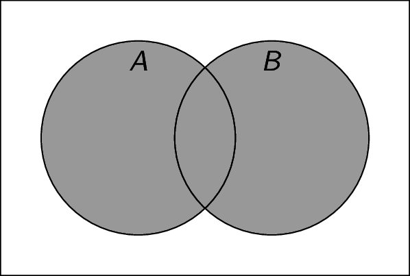
Union: Given two sets $A$ and $B$, the union $A \cup B$ is the set of all elements that are in either $A$ or $B$. For example, if $A = \{ 1,3,5 \}$ and $B = \{ 2,3,6 \}$, then $A \cup B = \{ 1,2,3,4,5,6 \}$. Note that $A \cup B = \{ x \;|\; (x \in A) \lor (x \in B) \}$.
-
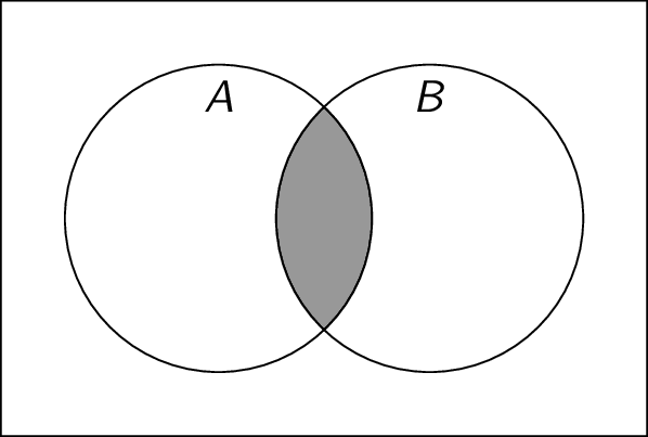
Intersection: Given two sets $A$ and $B$, the intersection $A \cap B$ is the set of all elements that are in both $A$ and $B$. For example, if $A = \{ 1,2,3,4 \}$ and $B = \{ 3,4,5,6 \}$, then $A \cap B = \{ 3,4 \}$. Note that $A \cap B = \{ x \;|\; (x \in A) \land (x \in B) \}$. We say that $A$ and $B$ are disjoint if $A \cap B = \emptyset$.
-
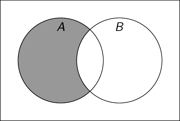
Difference: Given two sets $A$ and $B$, the difference $A \setminus B$ is the set of all elements that are in $A$ but not in $B$. For example, if $A = \{ 1,2,3,4 \}$ and $B = \{ 3,4 \}$, then $A \setminus B = \{ 1,2 \}$. Note that $A \setminus B = \{ x \;|\; (x \in A) \land (x \notin B) \}$. $A \setminus B$ is also denoted $A - B$.
-
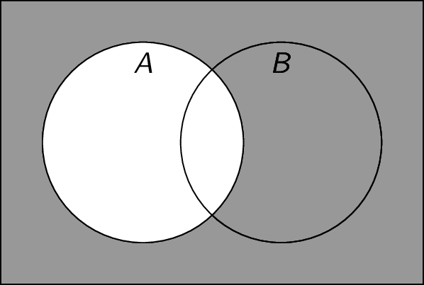
Complement: Given a set $A$, the complement $\overline{A}$ is the set of all elements that are not in $A$. To define this, we need some definition of the universe of all possible elements $U$. We can therefore view the complement as a special case of set difference, where $\overline{A} = U \setminus A$. For example, if $U = \mathbb{Z}$ and $A = \{ x \;|\; x \text{ is an odd integer} \}$, then $\overline{A} = \{ x \;|\; x \text{ is an even number} \}$. Note that $\overline{A} = \{ x \;|\; x \notin A \}$.
- Cartesian Product: Given two sets $A$ and $B$, the cartesian product $A \times B$ is the set of ordered pairs where the first element is in $A$ and the second element is in $B$. We have $A \times B = \{ (a,b) \;|\; a \in A \land b \in B \}$. For example, if $A = \{ 1,2,3 \}$ and $B = \{ a,b \}$, then $A \times B = \{ (1,a),(1,b),(2,a),(2,b),(3,a),(3,b) \}$.
Subsets
A set $A$ is a subset of a set $B$ if every element of $A$ is an element of $B$. We write $A \subseteq B$. Another way of saying this is that $A \subseteq B$ if and only if $\forall x\;(x \in A \rightarrow x \in B)$.
For any set S, we have:
-
$\emptyset \subseteq S$
Proof: Must show that $\forall x\;{(x \in \emptyset \rightarrow x \in S)}$. Since $x \in \emptyset$ is always false, the implication is always true. This is an example of a trivial or vacuous proof.
-
$S \subseteq S$
Proof: Must show that $\forall x\;{(x \in S \rightarrow x \in S)}$. Fix an element $x$. We must show that $x \in S \rightarrow x \in S$. This implication is equivalent to $x \in S \lor x \notin S$, which is a tautology. Therefore, by Universal Generalization, $S \subseteq S$.
Power Sets
The power set of a set $A$ is the set of all subsets of $A$, denoted $\mathcal{P}(A)$. For example, if $A = \{1,2,3\}$, then $\mathcal{P}(A) = \{ \emptyset, \{1\},\{2\},\{3\}, \{1,2\},\{2,3\},\{1,3\}, \{1,2,3\} \}$
Notice that $|\mathcal{P}(A)| = 2^{|A|}$.
Set Equality
Two sets are equal if they contain the same elements. One way to show that two sets $A$ and $B$ are equal is to show that $A \subseteq B$ and $B \subseteq A$:
\begin{array}{lll} A \subseteq B \land B \subseteq A & \equiv & \forall x\;{((x \in A \rightarrow x \in B) \land (x \in B \rightarrow x \in A))} \\ &\equiv & \forall x\;{(x \in A \leftrightarrow x \in B)} \\ &\equiv & A = B \\ \end{array}Note: it is not enough to simply check if the sets have the same size! They must have exactly the same elements. Remember, though, that order and repetition do not matter.
Membership Tables
We combine sets in much the same way that we combined propositions. Asking if an element $x$ is in the resulting set is like asking if a proposition is true. Note that $x$ could be in any of the original sets.
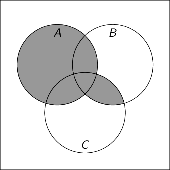
What does the set $A \cup (B \cap C)$ look like? We use $1$ to denote the presence of some element $x$ and $0$ to denote its absence.
\begin{array}{ccc|cc} A & B & C & B \cap C & A \cup (B \cap C) \\\hline 1 & 1 & 1 & 1 & 1 \\ 1 & 1 & 0 & 0 & 1 \\ 1 & 0 & 1 & 0 & 1 \\ 1 & 0 & 0 & 0 & 1 \\ 0 & 1 & 1 & 1 & 1 \\ 0 & 1 & 0 & 0 & 0 \\ 0 & 0 & 1 & 0 & 0 \\ 0 & 0 & 0 & 0 & 0 \\ \end{array}This is a membership table. It can be used to draw the Venn diagram by shading in all regions that have a $1$ in the final column. The regions are defined by the left-most columns.
We can also use membership tables to test if two sets are equal. Here are two methods of showing if $\overline{A \cap B} = \overline{A} \cup \overline{B}$:
- Showing each side is a subset of the other: \begin{array}{lll} x \in \overline{A \cap B} & \rightarrow & x \notin A \cap B \\ & \rightarrow & \neg(x \in A \cap B) \\ & \rightarrow & \neg(x \in A \land x \in B) \\ & \rightarrow & \neg(x \in A) \lor \neg(x \in B) \\ & \rightarrow & x \notin A \lor x \notin B \\ & \rightarrow & x \in \overline{A} \lor x \in \overline{B} \\ & \rightarrow & x \in \overline{A} \cup \overline{B} \end{array} \begin{array}{lll} x \in \overline{A} \cup \overline{B} & \rightarrow & x \notin A \lor x \notin B \\ & \rightarrow & \neg(x \in A) \lor \neg(x \in B) \\ & \rightarrow & \neg(x \in A \land x \in B) \\ & \rightarrow & \neg(x \in A \cap B) \\ & \rightarrow & x \notin A \cap B \\ & \rightarrow & x \in \overline{A \cap B} \end{array}
- Using membership tables: \begin{array}{ccc|ccccc} A & B & C & A \cap B & \bf \overline{A \cap B} & \overline{A} & \overline{B} & \bf \overline{A} \cup \overline{B} \\\hline 1 & 1 & 1 & 1 & \bf0 & 0 & 0 & \bf0 \\ 1 & 1 & 0 & 1 & \bf0 & 0 & 0 & \bf0 \\ 1 & 0 & 1 & 0 & \bf1 & 0 & 1 & \bf1 \\ 1 & 0 & 0 & 0 & \bf1 & 0 & 1 & \bf1 \\ 0 & 1 & 1 & 0 & \bf1 & 1 & 0 & \bf1 \\ 0 & 1 & 0 & 0 & \bf1 & 1 & 0 & \bf1 \\ 0 & 0 & 1 & 0 & \bf1 & 1 & 1 & \bf1 \\ 0 & 0 & 0 & 0 & \bf1 & 1 & 1 & \bf1 \\ \end{array} Since the columns corresponding to the two sets match, they are equal.
It is not sufficient to simply draw the Venn diagrams for two sets to show that they are equal: you need to show why your Venn diagram is correct (typically with a membership table).
There is an additional way to prove two sets are equal, and that is to use set identities. In the following list, assume $A$ and $B$ are sets drawn from a universe $U$.
- Identity Law: $A \cup \emptyset = A$, $A \cap U = A$
- Idempotent Law: $A \cup A = A$, $A \cap A = A$
- Domination Law: $A \cup U = U$, $A \cap \emptyset = \emptyset$
- Complementation Law: $\overline{\overline{A}} = A$
- Commutative Law: $A \cup B = B \cup A$, $A \cap B = B \cap A$
- Associative Law: $A \cup (B \cup C) = (A \cup B) \cup C$, $A \cap (B \cap C) = (A \cap B) \cap C$
- Distributive Law: $A \cap (B \cup C) = (A \cap B) \cup (A \cap C)$, $A \cup (B \cap C) = (A \cup B) \cap (A \cup C)$
- Absorption Law: $A \cup (A \cap B) = A$ and $A \cap (A \cup B) = A$
- De Morgan's Law: $\overline{A \cap B} = \overline{A} \cup \overline {B}$, $\overline{A \cup B} = \overline{A} \cap \overline {B}$
- Complement Law: $A \cup \overline{A} = U$, $A \cap \overline{A} = \emptyset$
- Difference Equivalence: $A \setminus B = A \cap \overline{B}$
Note the similarities to logical equivalences! Here are some examples of how to determine if two sets are equal:
- Is $(A \setminus C) \cap (B \setminus C)$ equal to $(A \cap B) \cap \overline{C}$? First, we can use a membership table: \begin{array}{ccc|cccccc} A & B & C & A \setminus C & B \setminus C & \bf (A \setminus C) \cap (B \setminus C) & A \cap B & \overline{C} & \bf (A \cap B) \cap \overline{C} \\\hline 1 & 1 & 1 & 0 & 0 & \bf0 & 1 & 0 & \bf0 \\ 1 & 1 & 0 & 1 & 1 & \bf1 & 1 & 1 & \bf1 \\ 1 & 0 & 1 & 0 & 0 & \bf0 & 0 & 0 & \bf0 \\ 1 & 0 & 0 & 0 & 0 & \bf0 & 0 & 1 & \bf0 \\ 0 & 1 & 1 & 0 & 0 & \bf0 & 0 & 0 & \bf0 \\ 0 & 1 & 0 & 0 & 1 & \bf0 & 0 & 1 & \bf0 \\ 0 & 0 & 1 & 0 & 0 & \bf0 & 0 & 0 & \bf0 \\ 0 & 0 & 0 & 0 & 0 & \bf0 & 0 & 1 & \bf0 \\ \end{array} Since the columns corresponding to the two sets match, they are equal. We can also use set identities: \begin{array}{llll} (A \setminus C) \cap (B \setminus C) & = & (A \cap \overline{C}) \cap (B \cap \overline{C}) & \text{Difference Equivalence} \\ & = & (A \cap B) \cap (\overline{C} \cap \overline{C}) & \text{Associative Law} \\ & = & (A \cap B) \cap \overline{C} & \text{Idempotent Law} \\ \end{array}
- Is $(A \setminus C) \cap (C \setminus B)$ equal to $A \setminus B$? Let's use some set identities: \begin{array}{llll} (A \setminus C) \cap (C \setminus B) & = & (A \cap \overline{C}) \cap (C \cap \overline{B}) & \text{Difference Equivalence} \\ & = & (A \cap \overline{B}) \cap (C \cap \overline{C}) & \text{Associative Law} \\ & = & (A \cap B) \cap \emptyset & \text{Complement Law} \\ & = & \emptyset & \text{Domination Law} \\ \end{array} Note that, in general, $A \setminus B \neq \emptyset$ (\eg, let $A=\{1,2\},B=\{1\}$). Therefore, these sets are not equal. (Note the similarity to finding truth settings that invalidate an argument!)
Functions
Suppose we want to map one set to the other: given an element of set $A$ (the input), return an element of set $B$ (the output).
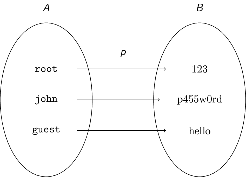
For example, suppose $A = \{ x \;|\; x \text{ is a user on our computer system} \}$ and $B = \{ x \;|\; x \text{ is a valid password}\}$. We might want to know, given a user, what is that user's password: the input is the user (from $A$) and the output is that user's password (from $B$).
Let $A$ and $B$ be two sets. A function from $A$ to $B$ is an assignment of exactly one element from $B$ to each element of $A$. We write $f(a) = b$ if $b \in B$ is the unique element assigned by the function $f$ to the element $a \in A$. If $f$ is a function from $A$ to $B$, we write $f : A \rightarrow B$.
It makes sense to model the password example above as a function because each user has exactly one password. Here are two other examples:
-
Suppose user root has password $\text{123}$, john has password $\text{p455w0rd}$, and guest has password $\text{hello}$. Call the password function $p$. Then $p(\texttt{root}) = \text{123}, p(\texttt{john}) = \text{p455w0rd}, p(\texttt{guest}) = \text{hello}$. We can also visualize $p$ as follows:
-
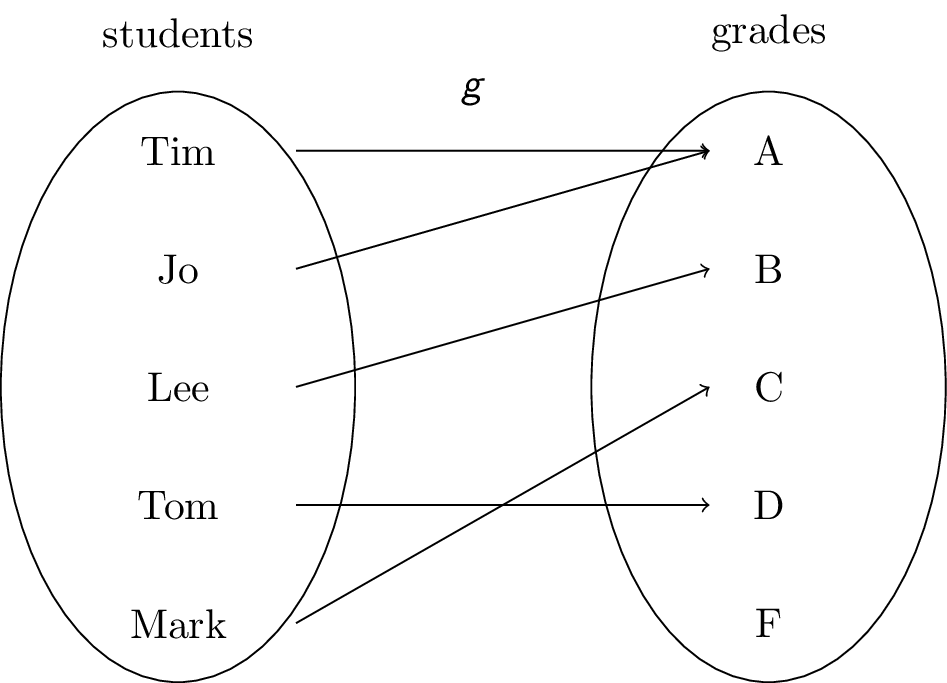
Consider a function $g$ that assigns a grade to each student in the class:
Functions can be specified in several ways:
- writing out each pair explicitly: $p(\texttt{root}) = \text{123}, \ldots$
- a diagram, as in the last two examples
- a formula: $f(x) = 2x^2 + 1$
Consider the function $f:A \rightarrow B$. We call $A$ the domain of $f$ and $B$ the codomain of $f$. Furthermore, if $f(a)=b$, then $b$ is the image of $a$ and $a$ is the preimage of $b$. The set of all images of elements of $A$ is called the range of $f$. For example:
-
In the grades example above:
- domain: $\{ \text{Tim}, \text{Jo}, \text{Lee}, \text{Tom}, \text{Mark} \}$
- codomain: $\{ \text{A}, \text{B}, \text{C}, \text{D}, \text{F} \}$
- range: $\{ \text{A}, \text{B}, \text{C}, \text{D} \}$
- $\text{A}$ is the image of $\text{Tim}$
- $\text{Tim}$ is a preimage of $\text{A}$
-
Let $f:\mathbb{Z} \rightarrow \mathbb{Z}$ be defined by $f(x)=x^2$.
- domain: $\mathbb{Z}$
- codomain: $\mathbb{Z}$
- range: $\{ x \;|\; x \text{ is a non-negative perfect square} \}$
If $S$ is a subset of the domain, we can also look at its image: the subset of $B$ that consists of the images of the elements in $S$: $f(S) = \{ f(s) \;|\; s \in S \}$. In the grades example above, $g(\{\text{Tim},\text{Jo},\text{Lee}\}) = \{\text{A},\text{B}\}$.
Notice that in the grades example, $\text{A}$ had two elements map to it, while $\text{F}$ had none. We can classify functions based on such situations.
Injectivity
A function $f$ is said to be injective or one-to-one if $(f(x) = f(y)) \rightarrow (x = y)$ for all $x$ and $y$ in the domain of $f$. The function is said to be an injection.
Recall that, by contraposition, $(f(x) = f(y)) \rightarrow (x=y)$ if and only if $(x \neq y) \rightarrow (f(x) \neq f(y))$.
Basically, this means that each element of the range has exactly one pre-image. Equivalently, each element of the codomain has at most one pre-image. In a function diagram, this means there is at most one incoming arrow to every element on the right hand side.
To show a function is injective:
- assume $f(x) = f(y)$ and show that $x=y$, or
- assume $x \neq y$ and show that $f(x) \neq f(y)$
To show a function is not injective, give an $x$ and $y$ such that $x \neq y$ but $f(x) = f(y)$.
Here are some examples:
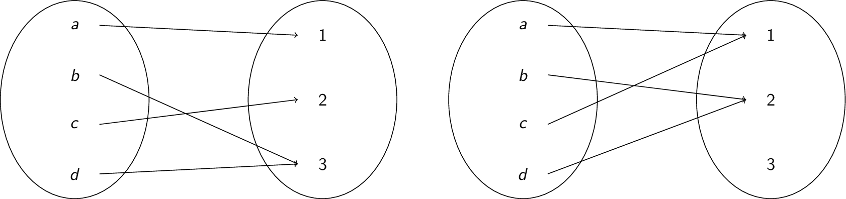
-
The function on the left is injective, but the function on the right is not:
- $f : \mathbb{Z} \rightarrow \mathbb{Z}$ defined by $f(x) = 3x+2$ is injective. To see this, assume $f(x) = f(y)$. Then: \begin{array}{rcl} 3x + 2 & = & 3y + 2 \\ 3x & = & 3y \\ x & = & y \end{array}
- The previous proof falls apart for $f(x) = x^2$: \begin{array}{rcl} x^2 & = & y^2 \\ \sqrt{x^2} & = & \sqrt{y^2} \\ \pm x & = & \pm y \end{array} which is not the same thing as $x = y$! Indeed, $f(x) = x^2$ is not injective since $f(1) = 1 = f(-1)$ and $1 \neq -1$.
Surjectivity
A function $f : A \rightarrow B$ is said to be surjective or onto if for every element $b \in B$, there is an element $a \in A$ such that $f(a) = b$. The function is said to be a surjection.
Basically, this means that every element of the codomain has a pre-image. Equivalently, the codomain and range are the same. In a function diagram, this means there is at least one incoming arrow to every element on the right hand side.
To show a function is surjective, start with an arbitrary element $b \in B$ and show what the preimage of $b$ could be: show an $a \in A$ such that $f(a) = b$. To show a function is not surjective, give a $b$ such that $f(a) \neq b$ for any $a \in A$.
Here are some examples:-
The function on the left is surjective, but the function on the right is not:

- $f : \mathbb{Z} \rightarrow \mathbb{Z}$ defined by $f(x) = x^2$ is not surjective, since there is no $x$ such that $x^2 = -1$ where $x$ is an integer.
- $f : \mathbb{R} \rightarrow \mathbb{R}$ defined by $f(x) = 3x+2$ is surjective. To see this, suppose we have image $3x+2=y$. To determine which pre-image gives this, observe that $3x+2 = y$ is the same as $3x = y-2$, which is the same as $x = (y-2)/3$. So, to get an output of $y$, give input $(y-2)/3$.
Notice that:
- injective $\leftrightarrow$ at most one image
- surjective $\leftrightarrow$ at least one image
If a function is both injective and surjective, then each element of the domain is mapped to a unique element of the codomain (range). A function that is both injective and surjective is bijective. Such a function is called a bijection.
To show a function is bijective, show:
- it is injective (using the above techniques)
- it is surjective (using the above techniques)
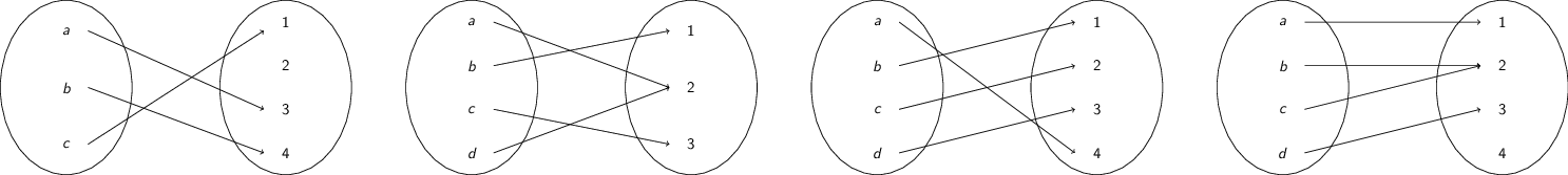
Remember to show both parts, since functions can be any combination of injective and surjective. For example, from left-to-right, the following functions are injective but not surjective, surjective but not injective, injective and surjective, and neither injective nor surjective:
Inverse of a Function
If a function $f$ is bijective, then $f$ is invertible. Its inverse is denoted $f^{-1}$ and assigns to $b \in B$ the unique element $a \in A$ such that $f(a) = b$: that is, $f^{-1}(b) = a \;\leftrightarrow\; f(a) = b$.
Inverses are not defined for functions that are not bijections.
- if $f$ is not injective, then some $b$ has two pre-images. Thus, $f^{-1}(b)$ would have more than one value and therefore $f^{-1}$ would not be a function
- if $f$ is not surjective, then some $b$ has no pre-image. Thus, $f^{-1}(b)$ would have no value and therefore $f^{-1}$ would not be a function
The inverse can be found by reversing the arrows in the diagram, or by isolating the other variable in the formula. Note that the inverse of $f : A \rightarrow B$ is $f^{-1} : B \rightarrow A$.
Here are some examples of functions and their inverses:
-
Consider the following function:
The function is injective and surjective and therefore bijective and invertible. We have $f^{-1}(1) = c, f^{-1}(2)=a, f^{-1}(3)=b$.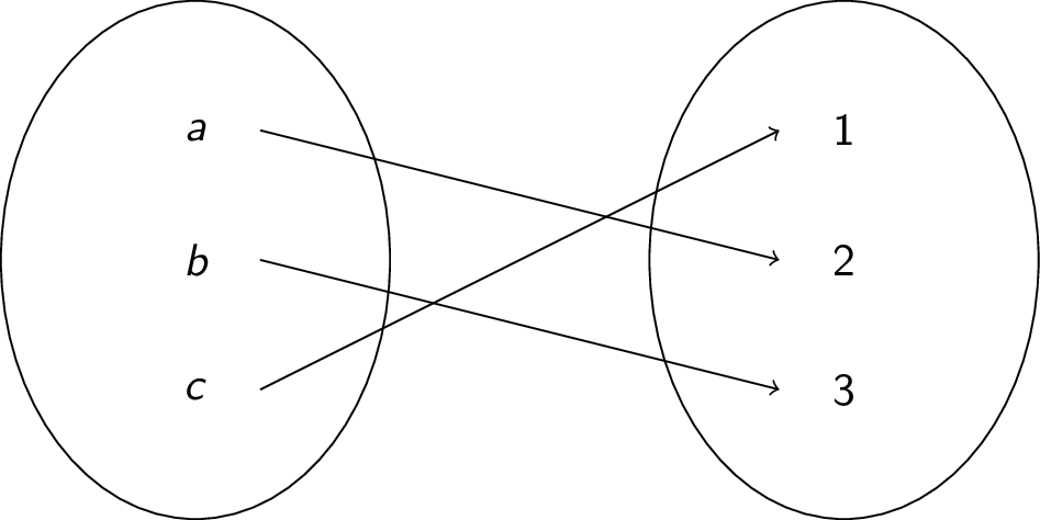
- $f : \mathbb{Z} \rightarrow \mathbb{Z}$ defined by $f(x) = 3x+2$ is bijective as we have already seen and is thus invertible. We know that $3x+2 = y \;\leftrightarrow\; 3x = y-2 \;\leftrightarrow\; x = \frac{y-2}{3}$. Therefore, $f^{-1}(x) = \frac{x-1}{3}$. (Note: it doesn't matter what variable you use, as long as you are consistent!)
- $f : \mathbb{Z} \rightarrow \mathbb{Z}$ defined by $f(x) = x^2$ is not invertible since it is not surjective.
Composition of Functions
Given two functions $f$ and $g$, we can use the output of one as the input to the other to create a new function $f(g(x))$. In this function, we evaluate $g$ with input $x$ and give the result to $f$ to compute the final output.
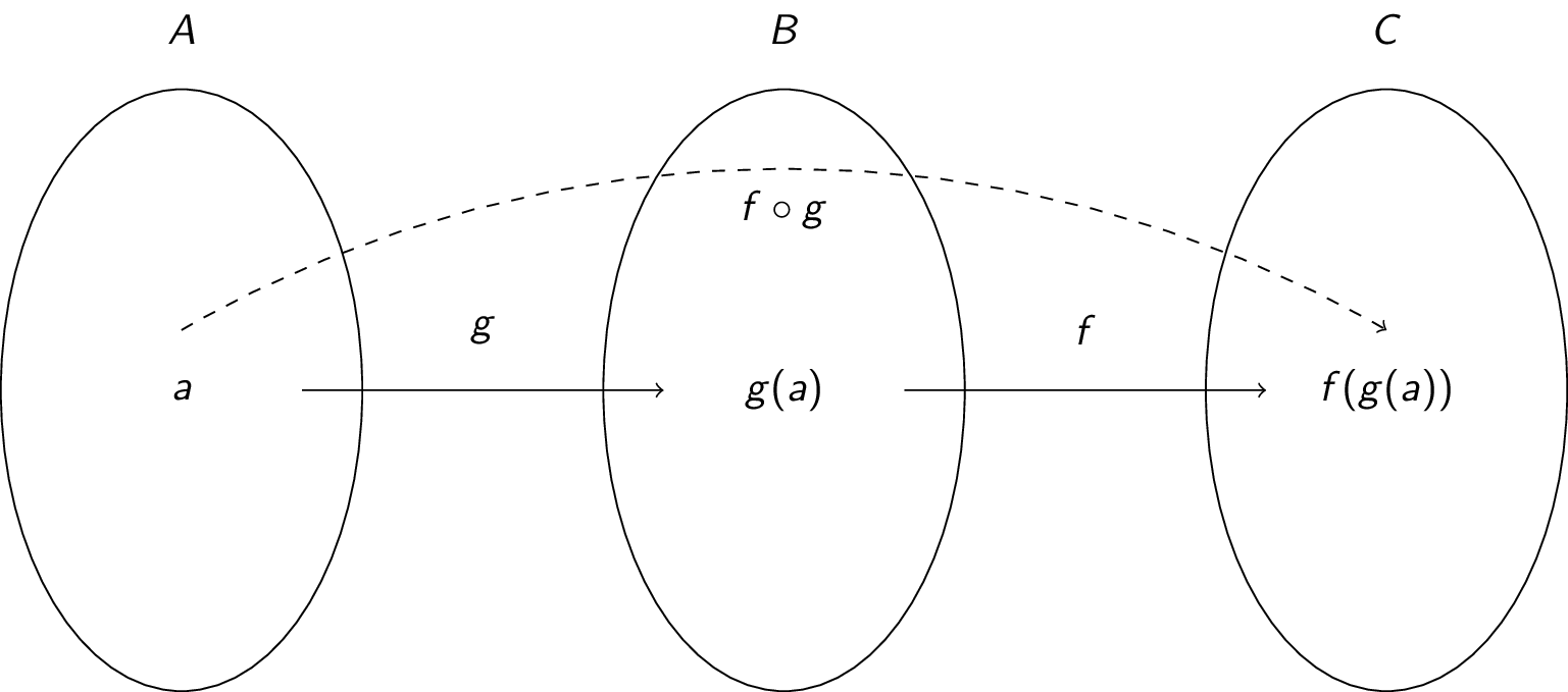
Let $f : B \rightarrow C$ and $g : A \rightarrow B$. The composition of $f$ and $g$ is denoted $f \circ g$ (read "$f$ follows $g$") and is defined as $(f \circ g)(x) = f(g(x))$. Note: for $f \circ g$ to be defined, the range of $g$ must be a subset of the domain of $f$.
Graphically, we have:
Here are some examples:
-
Define $g : \{a,b,c\} \rightarrow \{a,b,c\}$ and $f : \{a,b,c\} \rightarrow \{1,2,3\}$ in the following way:
- $g(a) = b, g(b) = c, g(c) = a$
- $f(a) = 3, f(b) = 2, f(c) = 1$
- $(f \circ g)(a) = f(g(a)) = f(b) = 2$
- $(f \circ g)(b) = f(g(b)) = f(c) = 1$
- $(f \circ g)(c) = f(g(c)) = f(a) = 3$
- Define $f:\mathbb{Z} \rightarrow \mathbb{Z}$ and $g:\mathbb{Z} \rightarrow \mathbb{Z}$ by $f(x) = 2x+3$ and $g(x)=3x+2$. Then: \begin{array}{rcl} (f \circ g)(x) &=& f(g(x)) \\ &=& f(3x+2) \\ &=& 2(3x+2)+3 \\ &=& 6x+4+3 \\ &=& 6x+7 \\ \end{array} and \begin{array}{rcl} (g \circ f)(x) &=& g(f(x)) \\ &=& g(2x+3) \\ &=& 3(2x+3)+2 \\ &=& 6x+9+2 \\ &=& 6x+11 \\ \end{array} In general, $f \circ g \neq g \circ f$!
One important case is composing a function with its inverse: Suppose $f(a) = b$. Then $f^{-1}(b)=a$, and:
- $(f^{-1} \circ f)(a) = f^{-1}(f(a)) = f^{-1}(b) = a$
- $(f \circ f^{-1})(b) = f(f^{-1}(b)) = f(a) = b$
Countable and Uncountable Sets
Notice that a bijection exists between two sets if and only if they have the same size. This allows us to reason about the sizes of infinite sets.
Consider $\mathbb{Z}^+ = \{1,2,\ldots\}$. We call a set countable if:
- it is finite, or
-
it has the same cardinality as $\mathbb{Z}^+$
- i.e., there is a bijection between it and $\mathbb{Z}^+$
- i.e., the elements of the set can be listed in order (first, second, third, ...)
Otherwise, the set is uncountable.
Here are some examples.
-
Are there more positive integers or positive odd integers?
This is the same as asking if the positive odd integers are countable, which is the same thing as asking if there is a bijection from $\mathbb{Z}^+$ to $\{1,3,5,7,9,\ldots\}$.
We claim $f(n)=2n-1$ is such a bijection. To see that $f$ is injective, suppose $f(n)=f(m)$; then $2n-1=2m-1$, so $2n=2m$, so $n=m$. To see that $f$ is surjective, suppose $t \in \{1,3,5,7,9,\ldots\}$; then $t=2k-1$, so $t=2k-1=f(k)$.
Since $f$ is injective and surjective, it is bijective. Therefore, there are equally many positive integers as positive odd integers!
-
Are there more positive integers or positive rational numbers?
We need $f : \mathbb{Z}^+ \rightarrow \mathbb{Q}^+$. Note that we just need to list the positive rational numbers in some way, since the first element can be $f(1)$, the second can be $f(2)$, and so on. How do we achieve such a listing?
A rational number has the form $p/q$. Since we are dealing with positive rational numbers, we have $p,q \in \mathbb{Z}^+$. The list consists of all positive rationals with $p+q=2$, then all positive rationals with $p+q=3$, then all positive rationals with $p+q=4$, and so on. We do not repeat a number if we encounter it again. Note that there are only a finite number of rationals with $p+q=k$ for a fixed $k$! The list looks like this:
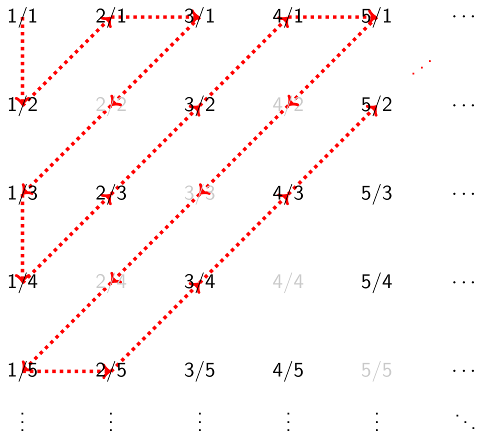
Therefore, there are equally many positive integers as positive rationals!
-
Are there more positive integers or real numbers?
This is the same as asking if $\mathbb{R}$ is countable. We will focus on an even "easier" problem: is the set $\{ x \;|\; (x \in \mathbb{R}) \land (0 \lt x \lt 1) \}$ (the set of real numbers strictly between $0$ and $1$) countable?
We will show that it is not countable. We prove this by contradiction, so suppose that it is countable. We can therefore list the elements:
- $0.d_{11}d_{12}d_{13}d_{14}\cdots$
- $0.d_{21}d_{22}d_{23}d_{24}\cdots$
- $0.d_{31}d_{32}d_{33}d_{34}\cdots$
- $0.d_{41}d_{42}d_{43}d_{44}\cdots$
- ...
Where $d_{ij} \in \{0,1,\ldots,9\}$.
Now, we come up with a real number $0 \lt x \lt 1$ that is not on this list. This will contradict the countability assumption! Consider $r = 0.d_1d_2d_3\cdots$, where $$ d_i = \begin{cases} 4 & \text{if } d_{ii} \neq 4\\ 5 & \text{if } d_{ii} = 4\\ \end{cases} $$
Notice that:
- $r \neq r_1$, since they differ in $d_1$ and $d_{11}$
- $r \neq r_2$, since they differ in $d_2$ and $d_{22}$
- $r \neq r_3$, since they differ in $d_3$ and $d_{33}$
- $\cdots$
Therefore, $r$ is not on the list, and we have a contradiction! Therefore, the real numbers are uncountable: they are bigger than $\mathbb{Z}^+$. (Why doesn't this argument work for the previous examples which were countable?)
Sequences and Sums
A sequence is a function from a subset of $\mathbb{Z}$ (usually $\{0,1,2,3,\ldots\}$ or $\{1,2,3,\ldots\}$) to a set $S$. We use $a_n$ to refer to the image of the integer $n$. We call $a_n$ a term of the sequence. The sequence itself is denoted $\{a_n\}$.
For example, if $a_n = 1/n$, then the sequence $\{a_n\}$ (beginning with $a_1$) is $a_1,a_2,a_3,\ldots$, or $1, 1/2, 1/3, 1/4, \ldots$.
A geometric sequence has the form $a, ar, ar^2, ar^3, \ldots, ar^n$ where $a$ is the initial term (a real number) and $r$ is the common ratio (also a real number). Typically, we think of such a sequence as starting with $n=0$ (since $ar^0 = a$). Here are some examples of geometric sequences:
- $\{b_n\}, b_n = (-1)^n$ has $a=-1,r=-1$ and looks like $ -1,1,-1,1,-1,\ldots$
- $\{c_n\}, c_n = 2 \times 5^n$ has $a=10,r=5$ and looks like $10,50,250,1250,\ldots$
- $\{d_n\}, d_n = 6 \times \left(\frac{1}{3}\right)^n$ has $a=2, r=1/3$ and looks like $2, 2/3, 2/9, 2/27,\ldots$
An arithmetic sequence has the form $a, a+d, a+2d, a+3d, \ldots, a+nd$ where $a$ is the initial term and $d$ is the common difference. Typically, we think of such a sequence as starting with $n=0$ (since $a+0d = a$). Here are some examples of arithmetic sequences:
- $\{s_n\}, s_n = -1+4n$ has $a=-1,d=4$ and looks like $-1,3,7,11,\ldots$
- $\{t_n\}, t_n = 7-3n$ has $a=7,d=-3$ and looks like $7,4,1,-2,\ldots$
One common operation on sequences is to compute a sum of certain portions of the sequence. Suppose we have $a_1,a_2,a_3,\ldots,a_m,a_{m+1},a_{m+2},\ldots,a_n,\ldots$ and we want to consider the sum from $a_m$ to $a_n$: $a_m + a_{m+1} + a_{m+2} + \cdots + a_n$. We can write this using sigma notation: $$ \sum_{i=m}^n a_i $$ where:
- $n$ is the upper limit
- $m$ is the lower limit
- $i$ is the index of summation
There is nothing special about using $i$; any (unused) variable would work!
Here are some examples of summations and sigma notation:
- The sum of the first $100$ terms of $\{a_n\}$ where $a_n = 1/n$ is $\displaystyle \sum_{i=1}^{100} a_i = \sum_{i=1}^{100} \frac{1}{i}$
- To compute the sum of the first $5$ squares, we have \begin{array}{rcl} \displaystyle \sum_{j=1}^5 j^2 &=& 1^2 + 2^2 + 3^2 + 4^2 + 5^2 \\ &=& 1 + 4 + 9 + 16 + 25 \\ &=& 55 \end{array}
Sometimes we might want to change the lower/upper limits without changing the sum. For example, suppose we want to change the sum $\displaystyle \sum_{j=1}^5 j^2$ to be written with lower limit $0$ and upper limit $4$. Then let $k=j-1$ to get $\displaystyle \sum_{j=1}^5 j^2 = \sum_{k=0}^4 (k+1)^2$
We can also split a sum up: $$\sum_{i=1}^n a_i = \sum_{i=1}^5 a_i + \sum_{i=6}^n a_i$$
This means that to exclude the first few terms of a sum, we can say: $$\sum_{i=6}^n a_i = \sum_{i=1}^n a_i - \sum_{i=1}^5 a_i$$
Summations can also be nested: $$\sum_{i=1}^n \sum_{j=1}^n ij$$
As an example, we compute $\sum_{i=1}^4 \sum_{j=1}^3 ij$: \begin{array}{rcl} \sum_{i=1}^4 \sum_{j=1}^3 ij &=& \sum_{i=1}^4 (1i + 2i + 3i) \\ &=& \sum_{i=1}^4 6i \\ &=& 6 + 12 + 18 + 24 \\ &=& 60 \end{array}
When every term is multiplied by the same thing, we can factor it out: $$\sum_{i=1}^n 6i = 6 \times \sum_{i=1}^n i$$
Here is another example of factoring, this time with a nested summation: $$\sum_{i=1}^4 \sum_{j=1}^3 ij = \sum_{i=1}^4 \left( i \times \sum_{j=1}^3 j \right) = \sum_{i=1}^4 6i = 6 \times \sum_{i=1}^4 i = 6 \times 10 = 60$$
You can also split over addition: $$\sum_{i=1}^n (i+2^i) = \sum_{i=1}^n i + \sum_{i=1}^n 2^i$$ This does not work for multiplication!
One useful tool is the sum of a geometric sequence, where $a,r \in \mathbb{R}$ and $r \neq 0$: $$ \sum_{j=0}^n ar^j = \begin{cases} \frac{ar^{n+1}-a}{r-1} & \text{if } r \neq 1 \\ (n+1)a & \text{if } r = 1 \\ \end{cases} $$
Why does this work? Let $S = \sum_{j=0}^n ar^j$. Then: \begin{array}{rcl} rS &=& r \sum_{j=0}^n ar^j \\ &=& \sum_{j=0}^n ar^{j+1} \\ &=& \sum_{k=1}^{n+1} ar^k \\ &=& \sum_{k=0}^n ar^k + (ar^{n+1} - a) \\ &=& S + (ar^{n+1} - a) \end{array}
Therefore, $rS = S + (ar^{n+1} - 1)$, so $S = \frac{ar^{n+1}-a}{r-1}$ as long as $r \neq 1$ (the case when $r=1$ is easy).
Here are some more useful summation formulas:
- $\sum_{k=1}^n k = \frac{n(n+1)}{2}$
- $\sum_{k=1}^n k^2 = \frac{n(n+1)(2n+1)}{6}$
- $\sum_{k=1}^n k^3 = \frac{n^2(n+1)^2)}{4}$
- $\sum_{k=0}^\infty x^k = \frac{1}{1-x}$ when $|x| \lt 1$
- $\sum_{k=1}^\infty kx^{k-1} = \frac{1}{(1-x)^2}$ when $|x| \lt 1$
Try to derive some of these yourself. For example, $\sum_{k=1}^n k = \frac{n(n+1)}{2}$ can be derived by letting $S = \sum_{k=1}^n k$ and observing that: \begin{array}{ccccccccccccc} S & = & 1 & + & 2 & + & 3 & + & \cdots & + & k-1 & + & k \\ S & = & n & + & n-1 & + & n-2 & + & \cdots & + & 2 & + & 1 \\\hline 2S & = & (n+1) & + & (n+1) & + & (n+1) & + & \cdots & + & (n+1) & + & (n+1) \\ \end{array}
Since there are $n$ terms, we have $2S = n(n+1)$, so $S = \frac{n(n=1)}{2} = \sum_{k=1}^n k$.
Algorithms
An algorithm is a finite set of precise instructions for solving a problem.
Here is an algorithm for outputting the largest number from a list of $n$ numbers. Such a number is called a maximum.
- set a temporary variable to the first number
- compare the next number to the temporary variable
- if it is larger, set the temporary variable to this number
- repeat step 2 until there are no more numbers left
- return the value of the temporary variable
Here is an algorithm for outputting the index of the number $x$ from an array of $n$ numbers. This is called a linear search.
-
look at the first element
- if it is equal to $x$, then return that index
-
look at the next element
- if it is equal to $x$, then return that index
- repeat step 2 until the end of the array is reached
- return not found
Sorting
For the sorting problem, we are given a list of elements that can be ordered (typically numbers) and wish to rearrange the list so that the elements are in non-decreasing order.
One algorithm that solves this problem is BubbleSort. It works by looking at pairs of elements in the list and "swapping" them whenever they are out of order. If this is done enough times, then the list will be in order! In pseudocode:
			BubbleSort$\left(a_1, a_2, \ldots, a_n\right)$
				for $i \gets 1$ to $n-1$
					for $j \gets 1$ to $n-i$
						if $a_j > a_{j+1}$
							swap $a_j$ and $a_{j+1}$
						end if
					end for
				end for
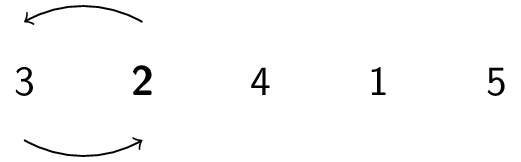
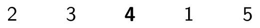
Here is how the BubbleSort algorithm works on the array $3,2,4,1,5$:
\begin{array}{c@{\hskip 0.5in}c@{\hskip 0.5in}c@{\hskip 0.5in}c} i=1 & i=2 & i=3 & i=4 \\\hline \underbrace{3,2}_\text{swap},4,1,5 & \underbrace{2,3}_\text{good},1,4,|5 & \underbrace{2,1}_\text{swap},3,|4,5 & \underbrace{1,2}_\text{good},|3,4,5 \\ 2,\underbrace{3,4}_\text{good},1,5 & 2,\underbrace{3,1}_\text{swap},4,|5 & 1,\underbrace{2,3}_\text{good},|4,5 \\ 2,3,\underbrace{4,1}_\text{swap},5 & 2,1,\underbrace{3,4}_\text{good},|5 & & \\ 2,3,1,\underbrace{4,5}_\text{good} & & & \\ \end{array}A natural question to ask is, "How long does this take?" The answer is: it depends! (On operating system, hardware, implementation, and many other things)
Another algorithm for sorting is InsertionSort.- it works by scanning the array left to right, looking for an element that is out of order
-
when such an element is found, it looks for where the element should go and places it there
- first, it must make room for the element, so it pushes the elements between where it was and where it should go back one
In pseudocode:
			InsertionSort$\left(a_1,a_2,\ldots,a_n\right)$
				for $j \gets 2$ to $n$
					$k \gets a_j$
					$i \gets j-1$
					while $i > 0$ and $a_i > k$
						$a_{i+1} \gets a_i$
						$i \gets i-1$
					end while
					$a_i \gets k$
				end for
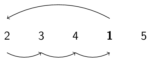
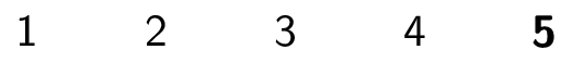
Here is how the InsertionSort algorithm works on the array $3,2,4,1,5$:
 |
 |
 |
 |
How long does this take? Again, it depends. But how does it compare to BubbleSort? (Assuming same hardware, operating system, etc.)
Analysis of Algorithms
To determine how "long" an algorithm takes, we need to know how long operations (such as additions, comparisons, etc.) take. To do this, we define a model of computation.
There are many such models. For now, let's say that comparisons (\ie, $\lt,\le,\gt,\ge,=,\neq$) take one time unit ("unit time"). The actual amount of time varies (with hardware, etc.), but we assume they all take the same time. This is generally a fair assumption.
The number of such operations is the time complexity of an algorithm. Typically, we will be interested in worst-case time complexity: the maximum number of operations performed.
Here are some examples of deriving time complexity:
-
Recall the algorithm to find the maximum number among a list of numbers. Here is the associated pseudocode:
						Maximum$\left(a_1,a_2,\ldots,a_n\right)$
							max $\gets a_1$
							for $i \gets 2$ to $n$
								if $a_i >$ max
									max $\gets a_i$
								end if
							end for
							return max
We use one comparison in each iteration of the for-loop (to ensure $i \le n$) and one comparison inside the for-loop to check if $a_i > $max. Since there are $n-1$ iterations, we do $2(n-1)$ comparisons. Note that one additional comparison is needed to exit the loop (the comparison for which $i \le n$ is false), so the total is therefore $2(n-1)+1 = 2n-1$ comparisons.
In this case, the worst case is the same as any case, since we always perform each of these comparisons regardless of the input.
-
What about linear search? Here is the associated pseudocode:
						LinearSearch$\left(x,a_1,a_2,\ldots,a_n\right)$
							for $i \gets 1$ to $n$
								if $a_i = x$
									return $i$
								end if
							end for
							return not found
As before, there is one comparison in each iteration of the loop, and then one comparison inside the loop. In the worst case, we have to perform every iteration of the loop (we do not find the element and return "early"), for a total of $2(n-1)+1 = 2n-1$ comparisons, just as in the last example.
Nevertheless, we could be "lucky" and find that $x=a_1$ after performing just $2$ comparisons. Generally, we are more interested in the worst case than the best case.
-
What about BubbleSort?
						BubbleSort$\left(a_1, a_2, \ldots, a_n\right)$
							for $i \gets 1$ to $n-1$
								for $j \gets 1$ to $n-i$
									if $a_j > a_{j+1}$
										swap $a_j$ and $a_{j+1}$
									end if
								end for
							end for
The outer loop goes through $n-1$ iterations and the inner loop goes through $n-i+1$ iterations. Each inner iteration does one comparison to check the loop condition and one comparison to check if $a_j > a_{j+1}$. One additional comparison is needed to leave the inner loop, and one additional comparison is needed to leave the outer loop. The total is therefore:
\begin{array}{rcl} && \displaystyle\sum_{i=1}^{n-1} \left( 1 + \left(\sum_{j=1}^{n-i} 2\right) + 1\right) + 1 \\ &=& \displaystyle\sum_{i=1}^{n-1} \left( 2(n-i-1+1) + 2\right) + 1 \\ &=& \displaystyle\sum_{i=1}^{n-1} (2n-2i + 2) + 1 \\ &=& \displaystyle 2n\sum_{i=1}^{n-1} 1 - 2\sum_{i=1}^{n-1} i + 2\sum_{i=1}^{n-1} 1 + 1 \\ &=& 2n(n-1) - 2\frac{n(n-1)}{2} + 2(n-1) + 1 \\ &=& n(n-1) + 2n - 2 + 1\\ &=& n^2 - n + 2n -2 + 1\\ &=& n^2 + n - 1\\ \end{array}Notice that this is always the same because there is no opportunity to be "lucky" and return early.
-
What about InsertionSort?
					InsertionSort$\left(a_1,a_2,\ldots,a_n\right)$
						for $j \gets 2$ to $n$
							$k \gets a_j$
							$i \gets j-1$
							while $i > 0$ and $a_i > k$
								$a_{i+1} \gets a_i$
								$i \gets i-1$
							end while
							$a_i \gets k$
						end for
We use one comparison per iteration of the outer loop (plus one to exit). The worst-case for the inner loop is that $i$ gets decremented from $j-1$ all the way to $0$, for a total of $j-1$ iterations with two comparisons each, plus two to exit. The total number of comparisons is therefore:
\begin{array}{rcl} && \displaystyle\sum_{j=2}^n \left(1 + \left(\sum_{i=1}^{j-1} 2\right) +2 \right) + 1\\ &=& \displaystyle \sum_{j=2}^n \left(1 + 2(j-1) + 2\right) + 1\\ &=& \displaystyle \sum_{j=2}^n \left(1 + 2j - 2 + 2\right) + 1\\ &=& \displaystyle \sum_{j=2}^n \left(2j+1\right) + 1\\ &=& \displaystyle \sum_{j=2}^n \left(2j\right) + \sum_{j=2}^n \left(1\right) + 1\\ &=& \displaystyle 2\sum_{j=2}^n j + (n-2+1) + 1\\ &=& \displaystyle 2\left(\frac{n(n+1)}{2} -1\right) + n - 2\\ &=& \displaystyle n(n+1) - 2 + n - 2\\ &=& \displaystyle n^2 + n - 2 + n - 2\\ &=& \displaystyle n^2 + 2n - 4\\ \end{array}Notice that this could be less if we are "lucky" and fewer iterations of the while-loop are required!
Notice that BubbleSort uses $n^2 + n - 1$ comparisons while InsertionSort uses $n^2 + 2n - 4$ comparisons. Therefore, BubbleSort uses fewer comparisons in the worst case.
But are these two functions really that different? Both have a $n^2$ term, which is much bigger than any (constant) fraction that they are multiplied by, and much bigger than any linear function of $n$ they are added to. As $n$ grows bigger and bigger, the $n^2$ part makes the biggest difference. In the worst case, these functions behave approximately the same.
Contrast this with finding the maximum and linear search: both use $2n-1$ comparisons. This is much faster than the two sorting algorithms, even though the leading term has coefficient $2$. This is because $n$ grows much more slowly than $n^2$. We care about large $n$.
Therefore, for the analysis of algorithms, we don't care too much about the exact function (since it is often too much work to find!) What matters is how fast the function grows.
Growth of Functions
The growth of a function is determined by the highest order term: if you add a bunch of terms, the function grows about as fast as the largest term (for large enough input values).
For example, $f(x) = x^2+1$ grows as fast as $g(x) = x^2 + 2$ and $h(x) = x^2+x+1$, because for large $x$, $x^2$ is much bigger than $1$, $2$, or $x+1$.
Similarly, constant multiples don't matter that much: $f(x)=x^2$ grows as fast as $g(x)=2x^2$ and $h(x)=100x^2$, because for large $x$, multiplying $x^2$ by a constant does not change it "too much" (at least not as much as increasing $x$).
Essentially, we are concerned with the shape of the curve:
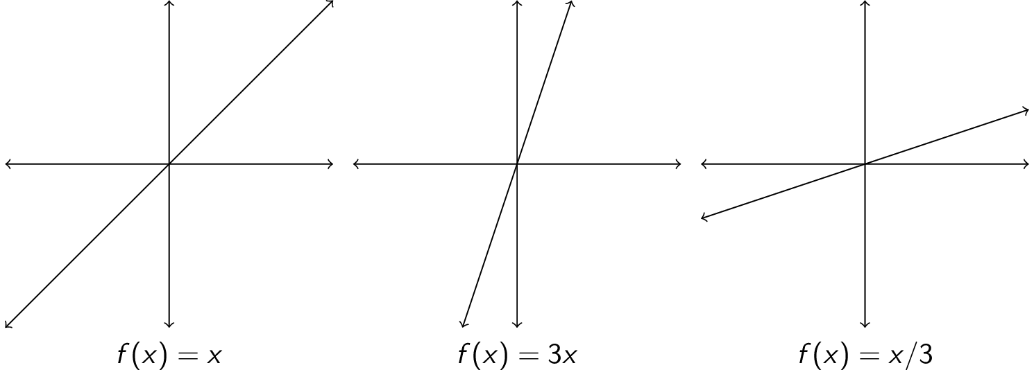
All three of these functions are lines; their exact slope/y-intercept does not matter.
Only caring about the highest order term (without constant multiples) corresponds to ignoring differences in hardware/operating system/etc. If the CPU is twice as fast, for example, the algorithm still behaves the same way, even if it executes faster.
Big-Oh Notation
Let $f$ and $g$ be functions from $\mathbb{Z} \rightarrow \mathbb{R}$ or $\mathbb{R} \rightarrow \mathbb{R}$. We say $f(x)$ is $O(g(x))$ if there are constants $c \gt 0$ and $k \gt 0$ such that $0 \le f(n) \le c \times g(n)$ for all $x \ge k$. The constants $c$ and $k$ are called witnesses. We read $f(x)$ is $O(g(x))$ as "$f(x)$ is big-Oh of $g(x)$". We write $f(x) \in O(g(x))$ or $f(x) = O(g(x))$ (though the former is more technically correct).
Basically, $f(x)$ is $O(g(x))$ means that, after a certain value of $x$, $f$ is always smaller than some constant multiple of $g$:
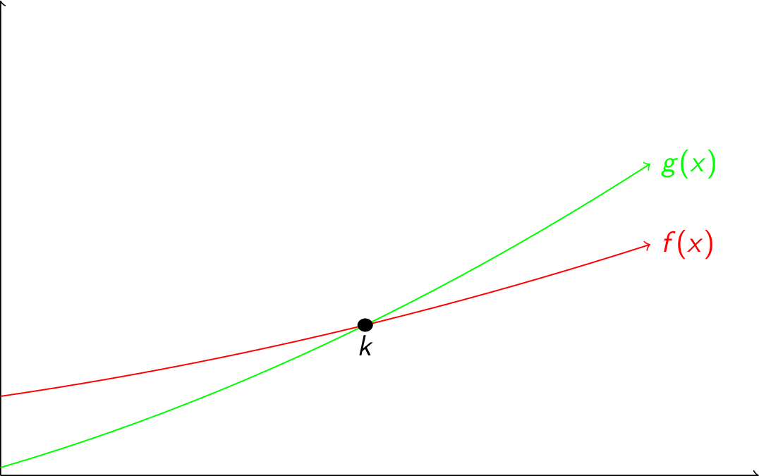
Here are some examples that use big-Oh notation:
- To show that $5x^2 + 10x + 3$ is $O(x^2)$: $$5x^2 + 10x + 3 \le 5x^2 + 10x^2 + 3x^2 = 18x^2$$ Each of the above steps is true for all $x \ge 1$, so take $c = 18$, $k=1$ as witnesses.
- To show that $5x^2 - 10x + 3$ is $O(x^2)$: $$5x^2 - 10x + 3 \le 5x^2 + 3 \le 5x^2 + 3x^2 = 8x^2$$ The first step is true as long as $10x > 0$ (which is the same as $x > 0$) and the second step is true as long as $x \ge 1$, so take $c=8$, $k=1$ as witnesses.
-
Is it true that $x^3$ is $O(x^2)$?
Suppose it is true. Then $x^3 \le cx^2$ for $x > k$. Dividing through by $x^2$, we get that $x \le c$. This says that "$x$ is always less than a constant", but this is not true: a line with positive slope is not bounded from above by any constant! Therefore, $x^3$ is not $O(x^2)$.
Typically, we want the function inside the Oh to be as small and simple as possible. Even though it is true, for example, that $5x^2+10x+3$ is $O(x^3)$, this is not terribly informative. Similarly, $5x^2+10x+3$ is $O(2x^2 + 11x + 3)$, but this is not particularly useful.
Here are some important big-Oh results:
-
If $f(x) = a_nx^n + a_{n-1}x^{n-1} + \cdots + a_1x + a_0$ where $a_n \gt 0$, then $f(x)$ is $O(x^n)$.
Proof: If $x>1$, then: \begin{array}{rcl} f(x) &= & a_nx^n + a_{n-1}x^{n-1} + \cdots + a_1x + a_0 \\ &\le & |a_n|x^n + |a_{n-1}|x^{n-1} + \cdots + |a_1|x + |a_0| \\ &\le & |a_n|x^n + |a_{n-1}|x^n + \cdots + |a_1|x^n + |a_0|x^n \\ &= & x^n(|a_n| + |a_{n-1}| + \cdots + |a_1| + |a_0|) \end{array} Therefore, take $c = |a_n| + |a_{n-1}| + \cdots + |a_1| + |a_0| \gt 0$ and $k = 1$.
- What is the sum of the first $n$ integers? $$1+2+3+\cdots+n \le n+n+n+\cdots+n = n \times n = n^2$$ Take $c=1,k=1$ to see that sum is $O(n^2)$. Notice that this agrees with the formula we derived earlier: $\sum_{i=1}^n i = n(n+1)/2$, which is $O(n^2)$.
- What is the growth of $n!$? \begin{array}{rcl} n! &=& n \times (n-1) \times (n-2) \times \cdots \times 2 \times 1 \\ &=& n \times n \times n \times \cdots n \\ &=& n^n \\ \end{array} Therefore, $n!$ is $O(n^n)$ with $c=k=1$
-
What is the growth of $\log n!$?
Take the logarithm of both sides of the previous equation to get $\log n! \le \log n^n$, so $\log n! \le n \log n$. Therefore, $\log n!$ is $O(n \log n)$ with $c=k=1$.
-
How does $\log_2 n$ compare to $n$?
We know that $n \lt 2^n$ (we will prove this later). Taking the logarithm of both sides, we have that $\log_2 n \lt \log_2 2^n = n$. So $\log_2 n$ is $O(n)$ with $c=k=1$.
When using logarithms inside big-Oh notation, the base does not matter. Recall the change-of-base formula: $\log_b n = \frac{\log n}{\log b}$. Therefore, as long as the base $b$ is a constant, it differs from $\log n$ by a constant factor.
Here are some common functions, listed from slowest to fastest growth: $$ O(1), O(\log n), O(n), O(n \log n), O(n^2), O(2^n), O(n!) $$ Caution: there are infinitely many functions between each element of this list!
Big-Omega Notation
As we saw above, big-Oh provides an upper bound for a function. To specify a lower bound, we use big-Omega notation.
Let $f$ and $g$ be functions from $\mathbb{Z} \rightarrow \mathbb{R}$ or $\mathbb{R} \rightarrow \mathbb{R}$. We say $f(x)$ is $\Omega(g(x))$ if there are constants $c \gt 0$ and $k \gt 0$ such that $0 \le c \times g(n) \le f(n)$ for all $x \ge k$. The constants $c$ and $k$ are called witnesses. We read $f(x)$ is $\Omega(g(x))$ as "$f(x)$ is big-Oh of $g(x)$". We write $f(x) \in \Omega(g(x))$ or $f(x) = \Omega(g(x))$ (though the former is more technically correct).
Basically, $f(x)$ is $\Omega(g(x))$ means that, after a certain value of $x$, $f$ is always bigger than some constant multiple of $g$:
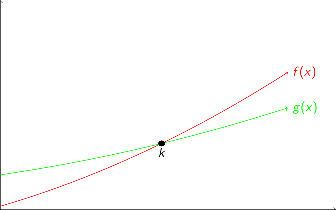
Here are some examples that use big-Omega notation:
- To show that $5x^3 + 3x^2 + 2$ is $\Omega(x^3)$: $$5x^3 + 3x^2 + 2 \ge 5x^3 \ge x^3$$ Therefore, take $c=k=1$.
- To show that $x^2 -3x + 4$ is $\Omega(x^2)$: \begin{array}{rcl} x^2 - 3x + 4 &=& \frac{1}{2}x^2 + \frac{1}{2}x^2 - 3x + 4 \\ &=& \frac{1}{2}x^2 + \left( \frac{1}{2}x^2 - 3x + 4 \right) \\ &\ge& \frac{1}{2}x^2 \end{array} The last step is true as long as $\frac{1}{2}x^2 - 3x + 4 \ge 0$, which is true when $x \gt 6$. Therefore, take $c = 1/2, k=6$.
-
Is it true that $3x+1$ is $\Omega(x^2)$?
Suppose it is true. Then $3x+1 \ge cx^2$ for $x \gt k$. Dividing through by $x^2$, we get that $3/x + 1/x^2 \ge c$. Notice that as $x$ gets bigger, the left hand side gets smaller, so this cannot be true. Therefore, $3x+1$ is not $\Omega(x^2)$.
- What is the sum of the first $n$ integers? \begin{array}{rcl} && 1+2+3+\cdots+n \\ &\ge& \left\lceil \frac{n}{2} \right\rceil + \left(\left\lceil \frac{n}{2} \right\rceil + 1\right) + \left(\left\lceil \frac{n}{2} \right\rceil + 2\right) + \cdots + n \\ &\ge& \left\lceil \frac{n}{2} \right\rceil + \left\lceil \frac{n}{2} \right\rceil + \cdots + \left\lceil \frac{n}{2} \right\rceil \\ &=& (n-\left\lceil \frac{n}{2} \right\rceil+1)\left\lceil \frac{n}{2} \right\rceil \\ &\ge& \left(\frac{n}{2}\right)\left(\frac{n}{2}\right) \\ &=& \frac{n^2}{4} \end{array} Therefore, take $c=1/4,k=1$ to show that the sum is $\Omega(n^2)$ (which matches with our formula for this sum).
Big-Theta Notation
In the previous example, we showed that $\sum_{i=1}^n i = \Omega(n^2)$. Earlier, we also showed that this sum is $O(n^2)$. We have special notation for such situations:
Let $f$ and $g$ be functions from $\mathbb{Z} \rightarrow \mathbb{R}$ or $\mathbb{R} \rightarrow \mathbb{R}$. We say $f(x)$ is $\Theta(g(x))$ if $f(x)$ is $O(g(x))$ and $f(x)$ is $\Omega(g(x))$. We read $f(x)$ is $\Theta(g(x))$ as "$f(x)$ is big-Theta of $g(x)$". We write $f(x) \in \Theta(g(x))$ or $f(x) = \Theta(g(x))$ (though the former is more technically correct).
It might be helpful to think of big-Oh/Omega/Theta as follows:
- $\le$ is to numbers as big-Oh is to functions
- $\ge$ is to numbers as big-Omega is to functions
- $=$ is to numbers as big-Theta is to functions
Induction
What is the sum of the first $n$ positive odd integers?
\begin{array}{rcl} n=1: & 1 & =1 \\ n=2: & 1+3 & =4 \\ n=3: & 1+3+5 & =9 \\ n=4: & 1+3+5+7 & =16 \end{array}So far, it seems like the pattern seems to be that the sum is $n^2$. But recognizing a pattern is not the same as a proof! How do we prove something is true for every $n$ (of which there are infinitely many)?
Imagine a long line of people, numbered $1,2,3,\ldots$. Suppose that whenever person $k$ is told something, thye tell person $k+1$. If I tell a secret to person $1$, what happens? $1$ tells $2$, $2$ tells $3$, $3$ tells $4$, and so on. So, after everyone is finished talking, everyone in the line knows what I said.
Let $P(n)$ denote the proposition "person $n$ knows the secret". The argument has premises $P(1)$ and $\forall k\;(P(k) \rightarrow P(k+1))$, with conclusion $\forall n\;P(n)$. Indeed, this is a valid argument:
\begin{array}{lll} 1. & P(1) & \\ 2. & \forall k\;(P(k) \rightarrow P(k+1)) & \therefore \forall n\;P(n) \\ \hline 3. & P(1) \rightarrow P(2) & \text{Universal Instantiation (2)} \\ 4. & P(2) & \text{Modus Ponens (1,3)} \\ 5. & P(2) \rightarrow P(3) & \text{Universal Instantiation (2)} \\ 6. & P(3) & \text{Modus Ponens (4,5)} \\ 7. & P(3) \rightarrow P(4) & \text{Universal Instantiation (2)} \\ 8. & P(4) & \text{Modus Ponens (6,7)} \\ & \vdots & \\ & P(1) \wedge P(2) \wedge \cdots & \text{Conjunction} \\ & \forall n\;P(n) & \text{Definition of } \forall \end{array}This gives us a proof technique to prove $\forall x\;P(x)$ when the universe of discourse is the natural numbers (starting at either $0$ or $1$). To summarize: $$ \left( P(1) \wedge \left(\forall k\;(P(k) \rightarrow P(k+1))\right) \right) \rightarrow \forall n\;P(n) $$
Why do we need (and like) this?
- before, we knew how to prove $\forall x\;(A(x) \rightarrow B(x))$, since we could pick an arbitrary $x$ and attempt a direct proof, but this doesn't always work (easily).
- now, we've converted the proof of $\forall n\;P(n)$ into an implication, so we can use a direct proof. By assuming something, we get more leverage.
Proving $P(1)$ is the basis step.
Proving $\forall k\;(P(k) \rightarrow P(k+1))$ is the inductive step.
- we will do this for some arbitrary $k$ (as in universal generalization). We do a direct proof, and so we call $P(k)$ the inductive hypothesis and assume that it is true in order to prove $P(k+1)$.
- we are not assuming $P(k)$ is true for all positive integers (this is circular reasoning); we are only assuming that $P(k)$ is true for some arbitrary $k$ in the same way we do for a regular direct proof of an implication
Let's show that our guess that the sum of the first $n$ positive odd integers is $n^2$ is correct. Let $P(n)$ denote "the sum of the first $n$ positive itnegers is $n^2$". We want to show $\forall n\;P(n)$ where the universe of discourse is the set of positive integers.
- Basis step: We must show $P(1)$. $P(1)$ says that the sum of the first $1$ positive odd integers is $1^2=1$. This is true.
- Inductive hypothesis: Assume $P(k)$ is true for an arbitrary $k$. This means that we assume that the sum of the first $k$ positive odd integers is $k^2$: $$ 1+3+5+\cdots+(2k-1)=k^2 $$ \item Inductive step: We must show that $P(k+1)$ is true using the inductive hypothesis. $P(k+1)$ says that the sum of the first $k+1$ positive odd integers is $(k+1)^2$, so let's look at the first $k+1$ positive odd integers: $$ 1+3+5+7+\cdots+(2k-1)+(2k+2) $$ By our inductive hypothesis, $1+3+5+\cdots+(2k-1)=k^2$, so the above expression can be rewritten as $$ k^2 + 2k + 1 $$ Factoring this, we obtain $(k+1)^2$. Therefore, the sum of the first $k+1$ positive odd integers is $(k+1)^2$, and so $P(k+1)$ is true under the assumption that $P(k)$ is true. Therefore, $P(k) \rightarrow P(k+1)$. Since $k$ was arbitrary, $\forall k\;(P(k) \rightarrow P(k+1))$ is true.
- By the basis step, we know that $P(1)$ is true. By the inductive step, we know that $\forall k\;(P(k) \rightarrow P(k+1))$ is true. Therefore, $P(1) \wedge \forall k\;(P(k) \rightarrow P(k+1))$ is true, and so by the principle of mathematical induction, $\forall n\;P(n)$ is true, as desired!
A few notes about doing proofs by mathematical induction:
- remember the structure: basis step, inductive hypothesis, inductive step
- label each part of the proof to help keep things in order
- it isn't necessary to define a propositional function, but you can (do not use one unless you state explicitly what it means!)
Induction works with inequalities, too. For example, here is a proof that $n \lt 2^n$ for all positive integers $n$.
- Basis step: If $n=1$, then we must show that $1 \lt 2^1 = 2$, which is true.
- Inductive hypothesis: Assume that $k \lt 2^k$ for some positive integer $k$.
- Inductive step: We must show that $k+1 \lt 2^{k+1}$. We have: $$ k+1 \lt 2^k + 1 \lt 2^k + 2^k \lt 2 \times 2^k = 2^{k+1} $$
Some more notes about doing proofs by mathematical induction:
- write out what you must do in the basis and inductive steps
- in the inductive step, you must prove $P(k+1)$: thus, you cannot assume it anywhere. Notice that in the last proof, we started with one side of the inequality and derived the other; we did not take $P(k+1)$ and simplify/change it to $P(k)$: that would be the wrong direction!
- how do you know when to use mathematical induction?
- look for statements like "for all positive integers" and other signs of universal quantification (where you don't get anywhere by just picking an arbitrary element and attempting universal generalization)
Induction can be used to show things other than equalities/inequalities. For example, here is a proof that $n^3 - n$ is divisble by $3$ for all positive integers $n$:
- Basis step: If $n=1$, then we must show that $1^3 - 1 = 1-1 = 0$ is divisible by $3$, which is true.
- Inductive hypothesis: Assume that $k^3 - k$ is divisible by $3$ for some positive integer $k$.
- Inductive step: We must show that $(k+1)^3 - (k+1)$ is divisible by $3$. We have: \begin{array}{rcl} (k+1)^3 - (k+1) &=& (k^3 + 3k^2 + 3k + 1) - (k+1) \\ &=& (k^3 - k) + (3k^2 +3k + 1 - 1) \\ &=& (k^3 - k) + 3(k^2 + k) \end{array} Notice that the $(k^3 - k)$ is divisible by $3$ by the inductive hypothesis, and $3(k^2+k)$ is divisble by $3$ because there is a factor of $3$. Since the sum of two numbers that are both divisible by $3$ is divisible by $3$, it must be true that $(k+1)^3 - (k+1)$ is divisible by $3$.
There is nothing special about starting at $1$. We can start at any integer $b$ (by using $b$ in our basis step). This will prove the proposition in question true over the universe of discourse $\{b,b+1,b+2,\ldots\}$.
Here is an example with a different basis step. We will prove that $2^0 + 2^1 + 2^2 + 2^3 + \cdots + 2^n = 2^{n+1} - 1$ for all non-negative integers.
- Basis step: The smallest non-negative integer is $0$. The left-hand side of the expression is $2^0 = 1$ and the right hand side is $2^1 - 1 = 1-1 = 0$, so the basis step has been proven.
- Inductive hypothesis: Assume $2^0 + 2^1 + 2^2 + 2^3 + \cdots + 2^k = 2^{k+1} - 1$ for some non-negative integer $k$.
- Inductive step: We must show that $2^0 + 2^1 + 2^2 + 2^3 + \cdots + 2^{k+1} = 2^{k+2} - 1$. We have: \begin{array}{rcl} && 2^0 + 2^1 + 2^2 + 2^3 + \cdots + 2^{k+1} \\ &=& (2^0 + 2^1 + 2^2 + 2^3 + \cdots + 2^k) + 2^{k+1} \\ &=& (2^{k+1} - 1) + 2^{k+1} \\ &=& 2 \times 2^{k+1} - 1 \\ &=& 2^{k+2} - 1 \end{array}
Recall the sum of a geometric sequence $\sum_{j=0}^n ar^j = a + ar + ar^2 + \cdots + ar^n$. We will prove that $\sum_{j=0}^n ar^j = \frac{ar^{n+1} - a}{r-1}$ when $r \neq 1$ and $n \ge 0$.
- Basis step: The statement says that $n \ge 0$, so our basis step occurs when $n=0$. The left-hand side is $\sum_{j=0}^0 ar^j = ar^0 = a$, and the right hand side is $$ \frac{ar^1 - a}{r-1} = \frac{ar-a}{r-1} = \frac{a(r-1)}{r-1} = a $$
- Inductive hypothesis: Assume that $\sum_{j=0}^k ar^j = \frac{ar^{k+1} - a}{r-1}$ for some non-negative integer $k$.
- Inductive step: We must show that $\sum_{j=0}^{k+1} ar^j = \frac{ar^{k+2} - a}{r-1}$. We have: \begin{array}{rcl} \displaystyle \sum_{j=0}^{k+1} ar^j &=& ar^{k+1} + \displaystyle\sum_{j=0}^{k} ar^j \\ &=& ar^{k+1} + \frac{ar^{k+1} - a}{r-1} \\ &=& \frac{(r-1)ar^{k+1}}{r-1} + \frac{ar^{k+1} - a}{r-1}\\ &=& \frac{ar^{k+1} - a + ar^{k+2} - ar^{k+1}}{r-1} \\ &=& \frac{ar^{k+2} - a}{r-1} \\ \end{array}
The $j$-th Harmonic number $H_j$ is defined as $H_j = 1 + \frac{1}{2} + \frac{1}{3} + \cdots + \frac{1}{j}$ when $j \ge 1$. We will prove that $H_{2^n} \ge 1 + \frac{n}{2}$ for non-negative integers $n$.
- Basis step: The statement says that $n \ge 0$, so our basis step occurs when $n=0$. The left-hand side is $H_{2^0} = 1$, and the right hand side is $1 + \frac{0}{2}$, so the statement is true.
- Inductive hypothesis: Assume that $H_{2^k} \ge 1 + \frac{k}{2}$ for some non-negative integer $k$.
- Inductive step: We must show that $H_{2^{k+1}} \ge 1 + \frac{k+1}{2}$. We have: \begin{array}{rcl} && H_{2^{k+1}} \\ &=& \frac{1}{1} + \frac{1}{2} + \frac{1}{3} + \cdots + \frac{1}{2^k} + \frac{1}{2^k + 1} + \cdots \frac{1}{2^{k+1}} \\ &\ge& \left(1 + \frac{k}{2}\right) + \underbrace{\frac{1}{2^k + 1} + \cdots \frac{1}{2^{k+1}}}_{2^k \text{ terms}} \\ &\ge& \left(1 + \frac{k}{2}\right) + 2^k \times \frac{1}{2^{k+1}} \\ &=& \left(1 + \frac{k}{2}\right) + \frac{1}{2} \\ &=& 1 + \frac{k+1}{2} \\ \end{array}
Recall that the size of the powerset of a set of size $n$ is $2^n$. We will now prove that this is true.
- Basis step: If $n=0$, then the set is empty and the only subset is $\emptyset$. Since $2^0 = 1$, the basis step is true.
- Inductive hypothesis: Assume that the size of the powerset of a set of size $k$ is $2^k$.
- Inductive step: We must show that the size of the powerset of a set of size $k+1$ is $2^{k+1}$.
Let $S$ be a set of $k+1$ elements. Write $S = S' \cup \{ a \}$ where $a \in S$ and $S' = S \setminus \{ a \}$.
- for each subset $X$ of $S'$, there are two subsets of $S$: $X$ and $X \cup \{ a \}$
- since each $X$ is distinct, each $X \cup \{a\}$ is distinct (since $a \notin S'$)
- since $|S| = k+1$, we know that $|S'| = k$. So there are $2^k$ subsets of $S'$ and each produces two subsets of $S$
- therefore, there are $2 \times 2^k = 2^{k+1}$ subsets of $S$
Recall the sum of the first $n$ positive integers: $\sum_{i=1}^n i = \frac{n(n+1)}{2}$. We will now prove that this is true.
- Basis step: When $n=1$, we have $\sum_{i=1}^1 i = 1 = \frac{1(2)}{2}$.
- Inductive hypothesis: Assume that $\sum_{i=1}^k i = \frac{k(k+1)}{2}$
- Inductive step: We must show that $\sum_{i=1}^{k+1} i = \frac{(k+1)(k+2)}{2}$. We have: \begin{array}{rcl} \sum_{i=1}^{k+1} i &=& \left(\sum_{i=1}^k i\right) + (k+1) \\ &=& \frac{k(k+1)}{2} + k + 1 \\ &=& \frac{k(k+1)}{2} + \frac{2(k+1)}{2} \\ &=& \frac{k(k+1) + 2(k+1)}{2} \\ &=& \frac{k^2 + 3k + 2}{2} \\ &=& \frac{(k+1)(k+2)}{2} \end{array}
Here is a proof that $2^n \lt n!$ for all positive integers $n \ge 4$:
- Basis step: When $n=4$, we have $2^4 = 16 \lt 24 = 4!$
- Inductive hypothesis: Assume that $2^k \lt k!$
- Inductive step: We must show that $2^{k+1} \lt (k+1)!$. We have: $$ 2^{k+1} = 2 \times 2^k \lt 2 \times k! \lt (k+1) \times k! = (k+1)! $$
Here is a proof of an extension of De Morgan's Law for sets: $\overline{\bigcap_{j=1}^n A_j} = \bigcup_{j=1}^n \overline{A_j}$, where $A_1,A_2,\ldots,A_n$ are sets and $n \ge 2$:
- Basis step: When $n=2$, we have $\overline{A_1 \cap A_2}$ on the left-hand side and $\overline{A_1} \cup \overline{A_2}$ on the right-hand side. This is precisely De Morgan's Law.
- Inductive hypothesis: Assume that $\overline{\bigcap_{j=1}^k A_j} = \bigcup_{j=1}^k \overline{A_j}$
- Inductive step: We must show that $\overline{\bigcap_{j=1}^{k+1} A_j} = \bigcup_{j=1}^{k+1} \overline{A_j}$. We have: \begin{array}{rcl} \overline{\bigcap_{j=1}^{k+1} A_j} &=& \overline{A_{k+1} \cap \bigcap_{j=1}^{k} A_j} \\ &=& \overline{A_{k+1}} \cup \overline{\bigcap_{j=1}^{k} A_j} \\ &=& \overline{A_{k+1}} \cup \bigcup_{j=1}^{k} \overline{A_j} \\ &=& \bigcup_{j=1}^{k+1} \overline{A_j} \\ \end{array}
Induction can also be used on other types of problems. Let $n$ be a positive integer. We will prove that any $2^n \times 2^n$ chessboard with one square removed can be tiled with L-shaped pieces that cover three squares:
- Basis step: When $n=1$, we consider $2 \times 2$ chessboards with one square removed. Here are the four possibilities, along with how they can be covered:
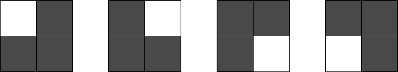
- Inductive hypothesis: Assume that any $2^k \times 2^k$ chessboard with one square removed can be tiled with L-shaped pieces.
-
Inductive step: We must show that any $2^{k+1} \times 2^{k+1}$ chessboard with one square removed can be tiled with L-shaped pieces.
Consider a $2^{k+1} \times 2^{k+1}$ chessboard with one square removed. Divide it in half in both directions to produce four $2^k \times 2^k$ chessboards. The missing square must be in one of these $2^k \times 2^k$ sub-boards. (Let's suppose it is the lower-right, but it does not matter which it is.)
By the inductive hypothesis, the lower-right can be tiled with one square removed. Now, pretend we remove the center squares as illustrated below. The other three sub-boards can be tiled by the inductive hypothesis, and the $2^{k+1} \times 2^{k+1}$ can be tiled by adding in one L-shaped piece in the center.
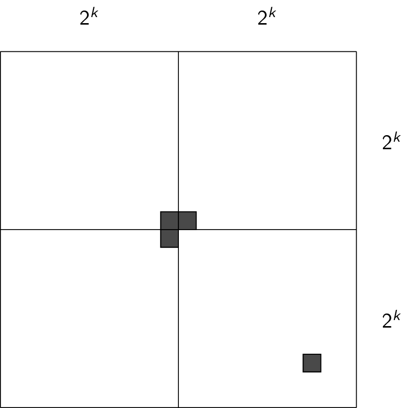
We will now prove that given $n \ge 2$ lines in the plane (no two of which are parallel), the total number of intersections is at most $\frac{n(n+1)}{2}$. (Recall that non-parallel lines intersect in exactly one point.)
- Basis step: If we have $n=2$ non-parallel lines, they intersect in exactly $1 \le \frac{1(2)}{2}$ point.
- Inductive hypothesis: Assume that the total number of intersects among $k$ non-parallel lines is at most $\frac{k(k+1)}{2}$.
- Inductive step: We must show that the total number of intersects among $k+1$ non-parallel lines is at most $\frac{(k+1)(k+2)}{2}$. Consider any collection of $k+1$ lines. Remove one line. By the inductive hypothesis, there are at most $\frac{k(k+1)}{2}$ intersections. Now add the removed line back. It can intersect each of the $k$ lines at most once, giving at most \begin{array}{rcl} \frac{k(k+1)}{2} + k &=& \frac{k^2 + k}{2} + \frac{2k}{2}\\ &=& \frac{k^2 + 3k}{2}\\ &\le& \frac{k^2 + 3k + 2}{2}\\ &=& \frac{(k+1)(k+2)}{2} \end{array} intersections in total.
Strong Induction
Recall that our argument when doing a proof by induction is the following:
\begin{array}{lll} 1. & P(1) & \\ 2. & \forall k\;(P(k) \rightarrow P(k+1)) & \therefore \forall n\;P(n) \\ \hline 3. & P(1) \rightarrow P(2) & \text{Universal Instantiation (2)} \\ 4. & P(2) & \text{Modus Ponens (1,3)} \\ 5. & P(2) \rightarrow P(3) & \text{Universal Instantiation (2)} \\ 6. & P(3) & \text{Modus Ponens (4,5)} \\ 7. & P(3) \rightarrow P(4) & \text{Universal Instantiation (2)} \\ 8. & P(4) & \text{Modus Ponens (6,7)} \\ & \vdots & \\ & P(1) \wedge P(2) \wedge \cdots & \text{Conjunction} \\ & \forall n\;P(n) & \text{Definition of } \forall \end{array}Notice that when we are proving $P(k+1)$, we know more than just $P(k)$; we actually know $P(1) \wedge P(2) \wedge \cdots P(k)$ is true! Therefore, it is valid to use $P(1) \wedge P(2) \wedge \cdots P(k)$ as our inductive hypothesis instead of simply $P(k)$. Using this inductive hypothesis is called strong induction and can (sometimes) make proofs simpler.
We will now look at some examples of proofs that use strong induction.
Consider a game: two players remove any number of matches they want from $1$ of $2$ piles. The player who removes the last match wins the game. The piles initially contain $n \ge 1$ matches each. We will prove that the player who goes second can always win.
- Basis step: If $n=1$, then the first player only take one match from one pile, leaving one match in the other. The second player then takes this match and wins.
- Inductive hypothesis: If there are $1 \le j \le k$ matches in each pile for some arbitrary $k$, the second player can always win.
- Inductive step: Suppose there are $k+1$ matches in each pile. The first player removes $j \ge 1$ matches from one pile, leaving $k+1-j \le k$. The second player then removes the same number of matches from the other pile. At this point, both piles have at most $k$ matches. Thus, by the inductive hypothesis, the second player can win. (Note: it could be that $j=k$, but then the second player can remove all matches in the other pile and win.)
Here is a proof that if $n \gt 1$, then $n$ can be written as a product of prime numbers.
- Basis step: If $n=2$, then $n$ is simply the product of itself, which is prime.
- Inductive hypothesis: Assume $2 \le j \le k$ can be written as a product of prime numbers for some arbitrary $k$.
- Inductive step: We must show that $k+1$ can be written as a product of prime numbers. We consider two cases:
- If $k+1$ is prime, then it is simply the product of itself, which is prime.
- If $k+1$ is not prime, then $k+1 = ab$ with $a \le a \le b \lt k+1$. By the inductive hypothesis, $a$ and $b$ are both products of primes, say $a = p_1p_2p_3\cdots$ and $b = q_1q_2q_3\cdots$. We have $$ k+1 = ab = p_1q_1 p_2q_2 p_3q_3 \cdots $$
Notice that in the previous proof, it is not straightforward to apply the original formulation of induction! For some proofs, both techniques apply equally well.
For example, we will prove that every amount of postage greater than or equal to 12¢ can be formed using 4¢ and 5¢ stamps.
- Induction:
- Basis step: 12¢ = 3 $\times$ 4¢
- Inductive hypothesis: Assume that a postage of $k$¢ can be formed using 4¢ and 5¢ stamps for some arbitrary $k \ge 12$
- Inductive step: We must show that a postage of $(k+1)$¢ can be formed. Consider postage for $k$¢ from inductive hypothesis. If one 4¢ stamp was used, replace it with a 5¢ stamp to get $(k+1)$¢. Otherwise, the postage for $k$¢ used only 5¢stamps. Since $k \ge 12$, at least 3 $\times$ 5¢ stamps were used. Therefore, if we replace 3 $\times$ 5¢ stamps with 4 $\times$ 4¢ stamps, we get $(k+1)$¢.
- Strong Induction
- Basis step: 12¢ = 3 $\times$ 4¢, 13¢ = 2 $\times$ 4¢ $+$ 1 $\times$ 5¢, 14¢ = 1 $\times$ 4¢ $+$ 2 $\times$ 5¢, 15¢ = 3 $\times$ 5¢
- Inductive hypothesis: Assume that a postage of $j$¢ can be formed for $12 \le j \le k$ for some arbitrary $k \ge 15$
- Inductive step: Use stamps for $(k-3)$¢ and add a $4¢$ stamp.
Note that the inductive step in the strong induction proof is only valid because we included the extra cases in the basis step.
Observe that using the usual method of induction resulted in a longer inductive step but shorter basis step, while strong induction resulted in a longer basis step but shorter inductive step.
Relations
Relations between elements of sets are very common. For example:
- sets of people related by the "father" relation
- employees related to companies by the "employed by" relation
- integers related to other integers by the "divisible by" relation
- (...and many other examples)
More formally: let $A$ and $B$ be sets. A binary relation from $A$ to $B$ is a subset of $A \times B$.
Therefore, a binary relation $R$ is just a set of ordered pairs. We write $aRb$ to mean $(a,b) \in R$ and $a \cancel{R} b$ to mean $(a,b) \notin R$. When $(a,b) \in R$, we say that "$a$ is related to $b$ by $R$".
Such relations are binary relations because $A \times B$ consists of pairs. In general, we can have relations that are subsets of $A \times B \times C \times \cdots$ to give us an $n$-ary relation. We concentrate on the binary case.
For example, let $A$ be the set of students at Carleton and $B$ be the set of courses at Carleton. Let $R$ be the "enrolled in" relation, so that $(a,b) \in R$ (that is, $aRb$) if student $a$ is enrolled in course $b$.
Note that you can think of all functions as relations (where the input is related to the output), but not vice versa (since a single element can be related to many others).
Sometimes, relations are between a set $A$ and itself: a subset of $A \times A$. In this case, we say the relation is on the set $A$.
Here are some more examples of relations:
-
Let $A = \{1,2,3,4\}$. What ordered pairs are in the relation $R = \{ (a,b) \;|\; a \text{ divides } b \}$?
$$ R = \{ (1,1), (1,2), (1,3), (1,4), (2,2), (2,4), (3,3), (3,4) \} $$
This can be represented several ways:
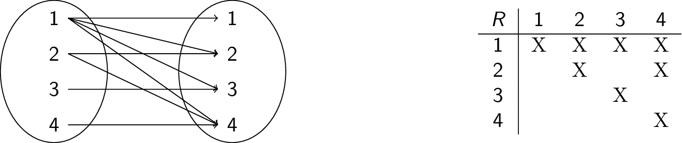
-
The following are relations on $\mathbb{Z}$:
- $R_1 = \{ (a,b) \;|\; a \le b \}$
- $R_2 = \{ (a,b) \;|\; a \gt b \}$
- $R_3 = \{ (a,b) \;|\; a = b \text{ or } a = -b \}$
- $R_4 = \{ (a,b) \;|\; a = b \}$
- $R_5 = \{ (a,b) \;|\; a = b+1 \}$
- $R_6 = \{ (a,b) \;|\; a+b \le 3 \}$
- $(1,1) \in R_1,R_3,R_4,R_6$
- $(1,2) \in R_1,R_6$
- $(2,1) \in R_2,R_5,R_6$
- $(1,-1) \in R_2,R_3,R_6$
- $(2,2) \in R_1,R_3,R_4$
Properties of Relations
Relations can have several properties which help to classify them.
-
Reflexivity: a relation $R$ on a set $A$ is reflexive if $(a,a) \in R$ for all $a \in A$.
For example, if $A = \{1,2,3,4\}$, then:
- $R_1 = \{ {\bf(1,1)},(1,2),{\bf(2,2)},(2,3),{\bf(3,3)},(3,1),{\bf(4,4)} \}$ is reflexive
- $R_2 = \{ (1,2),(2,3),(3,4) \}$ is not reflexive since $(1,1) \notin R_2$
- $R_3 = \{ (1,1),(2,2)(3,3),(1,4) \}$ is not reflexive since $(4,4) \notin R_3$
As another example, the "divides" relation is reflexive since $a = 1a$ for any integer $a$
- Symmetry: a relation $R$ on a set $A$ is called symmetric if $(a,b) \in R \rightarrow (b,a) \in R$ for all $a,b \in A$
-
Antisymmetry: a relation $R$ on a set $A$ is called antisymmetric if $((a,b) \in R \wedge (b,a) \in R) \rightarrow (a=b)$ for all $a,b \in A$.
Note: symmetry and antisymmetry are not mutually exclusive: a relation can have one, both, or neither. Consider the following relations on $\{1,2,3,4\}$:
-
$R_1 = \{ (1,1),(1,2),(2,1),(2,2),(3,4),(4,1),(4,4) \}$
- not symmetric: $(3,4) \in R_1$ but $(4,3) \notin R_1$
- not antisymmetric: $(2,1), (1,2) \in R_1$ but $1 \neq 2$
-
$R_2 = \{ (1,1),(1,2),(1,4),(2,1),(2,2),(3,3),(4,1) \}$
- symmetric
- not antisymmetric: $(2,1), (1,2) \in R_2$ but $1 \neq 2
-
$R_3 = \{ (2,1),(3,1),(3,2),(4,1),(4,2),(4,3) \}$
- not symmetric: $(2,1) \in R_3$ but $(1,2) \notin R_3$
- antisymmetric
-
$R_4 = \{ (1,1),(2,2) \}$
- symmetric
- antisymmetric
-
$R_1 = \{ (1,1),(1,2),(2,1),(2,2),(3,4),(4,1),(4,4) \}$
-
Transitivity: a relation $R$ on a set $A$ is called transitive if, for all $a,b,c \in A$,
$$((a,b) \in R \wedge (b,c) \in R) \rightarrow (a,c) \in R$$
For example, the following relations on $\mathbb{Z}$ are all transitive:
- $\{ (a,b) \;|\; a \le b \}$
- $\{ (a,b) \;|\; a \gt b \}$
- $\{ (a,b) \;|\; a = b \text{ or } a = -b \}$
- $\{ (a,b) \;|\; a = b \}$
whereas the following are not:
- $\{ (a,b) \;|\; a=b+1 \}$
- $\{ (a,b) \;|\; a+b \le 3 \}$
The "divides" relation is also transitive. Suppose $a|b$ and $b|c$. Then $b=ka$ and $c=lb$ for integers $k$ and $l$. Therefore, $c = lb = (lk)a$, so $a|c$.
Combining Relations
Relations are sets, so they can be combined the same way sets can be combined.
-
Let $A = \{1,2,3\}, B = \{ 1,2,3,4 \}$ and define the relations $R_1 = \{(1,1),(2,2),(3,3)\}$ and $R_2 = \{ (1,1),(1,2),(1,3),(1,4) \}$ from $A$ to $B$ can be combined as follows:
- $R_1 \cup R_2 = \{ (1,1),(1,2),(1,3),(1,4),(2,2),(2,3)\}$
- $R_1 \cap R_2 = \{ (1,1) \}$
- $R_1 \setminus R_2 = \{ (2,2),(3,3) \}$
- $R_2 \setminus R_1 = \{ (1,2),(1,3),(1,4) \}$
-
Let $R_1 = \{ (a,b) \;|\; a \lt b\}$ and $R_2 = \{ (a,b) \;|\; a \gt b \}$ be relations defined on $\mathbb{R}$.
- $R_1 \cup R_2 = \{(a,b) \;|\; a \lt b \text{ or } a \gt b\} = \{ (a,b) \;|\; a \neq b\}$
- $R_1 \cap R_2 = \{(a,b) \;|\; a \lt b \text{ and } a \gt b\} = \emptyset$
- $R_1 \setminus R_2 = R_1$
- $R_2 \setminus R_1 = R_2$
Remember the relations are like functions, so it makes sense to talk about their composition, too.
Let $R$ be a relation from set $A$ to set $B$. Let $S$ be a relation from set $B$ to set $C$. The composition of $R$ and $S$ is the relation consisting of ordered pairs $(a,c)$ where $a \in A$, $c \in C$ and there exists an element $b \in B$ such that $(a,b) \in R$ and $(b,c) \in S$. We write $S \circ R$ to denote this relation.
For example, if we have a relation $R$ from the set $\{1,2,3\}$ to the set $\{1,2,3,4\}$ and a relation $S$ from the set $\{1,2,3,4\}$ to the set $\{0,1,2\}$ defined as follows:
- $R = \{ (1,1),(1,4),(2,3),(3,1),(3,4) \}$
- $S = \{ (1,0),(2,0),(3,1),(3,2),(4,1) \}$
then $S \circ R = \{ (1,0),(1,1),(2,1),(2,2),(3,0),(3,1) \}$.
One special case of composition occurs when you compose a relation with itself. For example, let $R = \{ (a,b) \;|\; a \text{ is a parent of } b \}$ be defined on the set of all people. Then $R \circ R$ is the set of ordered pairs $(a,c)$ such that there exists a person $b$ so that $a$ is a parent of $b$ and $b$ is a parent of $c$, \ie, $a$ is a grandparent of $c$.
Of course, this produces a new relation which can be composed with $R$ again to produce the "is a great-grandparent of" relation.
As a shortcut, we write $R^2 = R \circ R$, $R^3 = (R \circ R) \circ R)$, and so on.
Let $R = \{ (1,1),(2,1),(3,2),(4,3) \}$. Then:
- $R^1 = R$
- $R^2 = \{ (1,1),(2,1),(3,1),(4,2) \}$
- $R^3 = \{ (1,1),(2,1),(3,1),(4,1) \}$
- $R^4 = R^3$
- $\vdots$
- $R^n = R^3$ for $n \ge 3$
Interestingly, we can understand transitivity in terms of composition: a relation $R$ on a set $A$ is transitive if and only if $R^n \subseteq R$ for $n \ge 1$.
- $(\leftarrow)$: Suppose $R^n \subseteq R$ for $n = 1,2,3,\ldots$. therefore, $R^2 \subseteq R$. Now, if $(a,b) \in R$ and $(b,c) \in R$, then $(a,c) \in R^2$. Since $R^2 \subseteq R$, we must have $(a,c) \in R$. Therefore, $R$ is transitive.
-
$(\rightarrow)$: We will use induction to prove this direction.
- Basis step: ($n=1$) If $R$ is transitive, then $R^1 = R$ is transitive.
- Inductive hypothesis: Assume $R^k \subseteq R$ for an arbitrary $k$.
- Inductive step: We want to show that $R^{k+1} \subseteq R$. Suppose that $(a,b) \in R^{k+1}$. Since $R^{k+1} = R^k \circ R$, there must exist an $x \in A$ such that $(a,x) \in R$ and $(x,b) \in R^k$. By the inductive hypothesis, $(x,b) \in R$. Since $R$ is transitive and $(a,x), (x,b) \in R$, we have that $(a,b) \in R$. Since $(a,b)$ was arbitrary, we have that $R^{k+1} \subseteq R$.
Reflexive Closure
Sometimes a relation does not have some property that we would like it to have: for example, reflexivity, symmetry, or transitivity.
How do we add elements to our relation to guarantee the property? Ideally, we'd like to add as few new elements as possible to preserve the "meaning" of the original relation.
We first consider making a relation reflexive. This is called the reflexive closure. Suppose we have a relation $R$ on a set $A$ and want to make it reflexive. We need to ensure that $(a,a)$ is in the relation for all $a \in A$. We also do not wish to add anything extra.
Define $\Delta = \{ (a,a) \;|\; a \in A \}$. The reflexive closure of $R$ is $R \cup \Delta$.
For example, the reflexive closure of $R = \{ (a,b) \;|\; a \lt b \}$ on the set of integers is the relation
$$R \cup \Delta = \{ (a,b) \;|\; a \lt b \} \cup \{ (a,a) \;|\; a \in \mathbb{Z} \} = \{ (a,b) \;|\; a \le b \}$$Symmetric Closure
For the symmetric closure, we want to ensure that $(b,a)$ is in the closure relation whenever $(a,b)$ is in the original relation.
Define $R^{-1} = \{ (b,a) \;|\; (a,b) \in R \}$. The symmetric closure of $R$ is $R \cup R^{-1}$.
For example, the symmetric closure of $R = \{ (a,b) \;|\; a \lt b \}$ on the set of integers is the relation
$$R \cup R^{-1} = \{ (a,b) \;|\; a \lt b \} \cup \{ (b,a) \;|\; a \gt b \} = \{ (a,b) \;|\; a \neq b \}$$Transitive Closure
Consider $R = \{ (1,3),(1,4),(2,1),(3,2) \}$ on $A = \{1,2,3,4\}$. This is not a transitive relation: it is missing $\{(1,2),(2,3),(2,4),(3,1) \}$. Let's try adding them and calling the new relation $R'$:
$$R' = \{ (1,3),(1,4),(2,1),(3,2),(1,2),(2,3),(2,4),(3,1) \}$$Unfortunately, this relation is still not transitive: $(3,1) \in R'$ and $(1,4) \in R'$, but $(3,4) \notin R'$. It seems we will need to do a bit more work.
Recall that if we compose $R$ with itself, then we get the elements $(a,c)$ where $(a,b) \in R$ and $(b,c) \in R$ for some $b$. We need these elements for transitivity, so add them to $R$. As we saw above, this might not be enough, so we repeat this.
How any times do we repeat? This is the same as asking how many intermediate elements we could find. Since there are $|A|$ possible intermediate elements, we might need to do as many as $|A|$ compositions.
Therefore, the transitive closure of $R$ over a set $A$ is
$$R \cup R^2 \cup R^3 \cup \cdots \cup R^{|A|}$$Here is an example of computing the transitive closure:
-
Let $R = \{ (1,1),(1,3),(2,2),(3,1),(3,2) \}$ over the set $A = \{1,2,3\}$. Then:
- $R^1 = R$
- $R^2 = \{ (1,1),(1,2),(1,3),(2,2),(3,1),(3,2),(3,3) \}$
- $R^3 = \{ (1,1),(1,2),(1,3),(2,2),(3,1),(3,2),(3,3) \}$
It turns out we can view this another way if we look at the matrix representation. Given a matrix representations $M_R$ and $M_S$ for the relations $R$ and $S$, the matrix representation of $S \circ R$ is $M_R \odot M_S$, where $\odot$ denotes the join operation. This operation is identical to matrix multiplication, but any non-zero entries are simply written as ones.
The matrix representation of $R$ in the previous example is $$ M_R = \begin{bmatrix} 1 & 0 & 1 \\ 0 & 1 & 0 \\ 1 & 1 & 0 \\ \end{bmatrix} $$
Therefore, we have: $$ M_{R^2} = M_R \odot M_R = \begin{bmatrix} 1 & 1 & 1 \\ 0 & 1 & 0 \\ 1 & 1 & 1 \\ \end{bmatrix} $$ and $$ M_{R^3} = M_{R^2} \odot M_R = \begin{bmatrix} 1 & 1 & 1 \\ 0 & 1 & 0 \\ 1 & 1 & 1 \\ \end{bmatrix} $$
We now take the union of these matrices by taking the logical-or of each entry: $$ \begin{bmatrix} 1 & 0 & 1 \\ 0 & 1 & 0 \\ 1 & 1 & 0 \\ \end{bmatrix} \vee \begin{bmatrix} 1 & 1 & 1 \\ 0 & 1 & 0 \\ 1 & 1 & 1 \\ \end{bmatrix} \vee \begin{bmatrix} 1 & 1 & 1 \\ 0 & 1 & 0 \\ 1 & 1 & 1 \\ \end{bmatrix} = \begin{bmatrix} 1 & 1 & 1 \\ 0 & 1 & 0 \\ 1 & 1 & 1 \\ \end{bmatrix} $$
As we would expect, this is the matrix representation of $\{ (1,1),(1,2),(1,3),(2,2),(3,1),(3,2),(3,3) \}$; the same answer we computed previously.
Equivalence Relations
We intuitively know what it means to be "equivalent", and some relations satisfy these intuitions, while others do not.
Consider the usual "$=$" relation. This is a perfectly good relation: we usually write $1=1$, for example, but can define $R = \{ (a,b) \;|\; a=b \}$ on $\mathbb{Z}$, and write $(1,1) \in R$ or $1R1$.
Why do we say the "$=$" relation expresses equivalence?
- anything is equivalent to itself (reflexive)
- if $a=b$ then $b=a$ (symmetric)
- if $a=b$ and $b=c$, then $a=c$ (transitive)
Other examples include logical equivalence, set equivalence, and many others.
A relation is an equivalence relation if it is reflexive, symmetric and transitive.
To show something is an equivalence relation, just show that it has all of these properties. To show a relation is not an equivalence relation, show it does not satisfy at least one of these properties.
Here are some examples of determining if relations are equivalence relations:
-
$R = \{ (a,b) \;|\; a=b \text{ or } a = -b \}$ over $\mathbb{Z}$
- reflexive: $a = a$, so $(a,a) \in R$
- symmetric: assume $(a,b) \in R$. Then $a=b$ or $a=-b$. If $a=b$, then $b=a$ so $(b,a) \in R$. If $a = -b$, then $b = -a$, so $(b,a) \in R$.
-
transitive: assume $(a,b) \in R$ and $(b,c) \in R$. Then $a=b$ or $a=-b$ and $b=c$ or $b=-c$.
- if $a=b$ and $b=c$, then $a=c$ so $(a,c) \in R$
- if $a=b$ and $b=-c$, then $a=-c$ so $(a,c) \in R$
- if $a=-b$ and $b=c$ then $-b=-c$, so $a=-b=-c$, so $(a,c) \in R$
- if $a=-b$ and $b=-c$ then $-b=c$, so $a=-b=c$, so $(a,c) \in R$
-
$R = \{ (a,b) \;|\; m \text{ divides } a-b \}$ (for some $m \in \mathbb{Z}^+$) over $\mathbb{Z}$
- reflexive: $m$ divides $a-a=0$ since $0 = 0 \times m$
- symmetric: assume $(a,b) \in R$. Then $m$ divides $a-b$. So $a-b = km$ for some integer $k$. Therefore, $-(a-b) = -km$, so $b-a = (-k)m$ and $m$ divides $b-a$, so $(b,a) \in R$.
- transitive: assume $(a,b) \in R$ and $(b,c) \in R$. Then $a-b = k_1m$ and $b-c = k_2m$. Adding these two equations together gives $(a-b)+(b-c) = k_1m + k_2m$, or $a-c = (k_1+k_2)m$, so $m$ divides $a-c$ and $(a,c) \in R$
-
$R$ is a relation on sets of strings of English letters such that $(a,b) \in R$ iff $a$ and $b$ have the same length
- reflexive: any string has the same length as itself
- symmetric: if $(a,b) \in R$ then the length of $a$ is the same as the length of $b$, $(b,a) \in R$ as well
- transitive: assume $(a,b) \in R$ and $(b,c) \in R$. Then the lengths of $a$, $b$, and $c$ are all the same. In particular, the lengths of $a$ and $c$ are the same, so $(a,c) \in R$
-
Is the divides relation on the integers an equivalence relation?
- reflexive: $a|a$ since $a = 1 \times a$
- transitive: if $a|b$ and $b|c$, we know that $b=k_1a$ and $c=k_2b$, so $c = k_1b = k1(k_2)a = (k_1k_2)a$, so $a|c$
- symmetric: the relation is not symmetric since $2|4$ but $4$ does not divide $2$
-
$R = \{ (a,b) \;|\; |a-b| \lt 1 \}$ over $\mathbb{R}$
- reflexive: $a-a = 0 \lt 1$
- symmetric: if $(a,b) \in R$ then $|a-b| \lt 1$. Since $|a-b| = |b-a|$, we have that $|b-a| \lt 1$
- transitive: if $x = 2.8$, $y=1.9$, $z=1.1$, then
- $|x-y| = |2.8-1.9| = 0.9 \lt 1$, so $(x,y) \in R$
- $|y-z| = |1.9-1.1| = 0.8 \lt 1$, so $(y,z) \in R$
- $|x-z| = |2.8-1.1| = 1.7 \ge 1$, so $(x,z) \notin R$
Equivalence Classes
Equivalence relations naturally partition the elements of the set they are defined on into several classes.
For example, let $R = \{ (a,b) \;|\; a \text{ got the same grade as } b \text{ in this course} \}$ over the set of students in this course. It is clear that $R$ is an equivalence relation. Observe that it also partitions the students in this course into classes: A+, A, A-, B+, and so on.
Let $R$ be an equivalence relation on a set $A$. The set of all elements related by $R$ to $a$ is called the equivalence class of $a$ and is denoted $[a]_R$ (or $[a]$ when $R$ is clear from context): $$[a]_R = \{ b \;|\; (a,b) \in R \}$$
If $b \in [a]_R$, then $b$ is called a representative of the equivalence class. Any member of the class can be chosen to be a representative.
Here are some examples of working with equivalence classes:
- Recall $R = \{ (a,b) \;|\; a=b \text{ or } a=-b \}$ is an equivalence relation over $\mathbb{Z}$. An integer is equivalent to itself and its negative, so we have $[a] = \{a,-a\}$. In particular, $[1] = \{1,-1\}, [2] = \{2,-2\}$, and so on. Note that $[0] = \{0\}$
- Let $R = \{ (a,b) \;|\; a \text{ and } b \text{ have the same first letter} \}$ over the set of English words. This is an equivalence relation, and they equivalene classes are all words starting with "a", all words starting with the letter "b", and so on.
In the grades example we saw before, the equivalence classes were the students who achieved the same grade. Notice that this is a partition: two equivalence classes are either equal or disjoint, and the union of all equivalence classes is the set over which the relation is defined.
This works the other way, too: given a partition of a set $A$, we can always construct an equivalence relation $R$ on $A$ with those equivalence classes.
-
Suppose we partition $A = \{1,2,3,4,5,6\}$ into $A_1 = \{1\}, A_2 = \{2,3\}, A_3 = \{4,5,6\}$. Define an equivalence relation on $A$ with equivalence classes $A_1,A_2,A_3$.
To do this, we simply define the relation to ensure that each element in subset is related to every other element in the subset:
- $R_1 = \{ (a,b) \;|\; a,b \in A_1 \} = \{ (1,1) \}$
- $R_2 = \{ (a,b) \;|\; a,b \in A_2 \} = \{ (2,2),(2,3),(3,2),(3,3) \}$
- $R_3 = \{ (a,b) \;|\; a,b \in A_3 \} = \{ (4,4), (4,5), (4,6), (5,4), (5,5), (5,6),(6,4), (6,5), (6,6) \}$
Taking the union $R_1 \cup R_2 \cup R_3$ gives the desired relation $R$.
Partial Orders
A relation $R$ on a set $A$ is called a partial ordering or partial order if it is reflexive, antisymmetric, and transitive. A set $A$ together with a partial order $R$ on that set is called a partially ordered set or poset and is denoted $(A,R)$. Members of $A$ are called elements of the poset.
Here are some examples:
-
The $\ge$ relation on $\mathbb{Z}$ is a partial order:
- reflexive: $a \ge a$ for all $a \in \mathbb{Z}$
- antisymmetric: if $a \ge b$ and $b \ge a$, then $a=b$
- transitive: if $a \ge b$ and $b \ge c$, then $a \ge c$
-
We saw in the last section that the "divides" relation on $\mathbb{Z}^+$ is reflexive and transitive. Is it antisymmetric?
Yes. If $a|b$ and $b|a$, then $b = ak_1$ and $a = bk_2$, so $b = bk_1k_2$, so $k_1k_2 = 1$. Since $k_1, k_2 \in \integers^+$, $k_1 = k_2 = 1$, and so $b=ak_1=a$.
In a partial order, we cannot always compare two elements. The elements $a,b$ of a poset $(S,\preceq)$ are comparable if either $a \preceq b$ or $b \preceq a$. When neither is true, they are incomparable.
- In the "divides" relation, $5$ does not divide $7$ and $7$ does not divide $5$, so they are incomparable. However, $2$ divides $4$ so $2$ and $4$ are comparable.
- In the $\le$ relation, we always have $a \le b$ or $b \le a$, so every pair of elements is comparable.
The fact that we can have incomparable elements is why the relations are called partial orderings.
If $(S,\preceq)$ is a poset and every two elements of $S$ are comparable, $S$ is called a totally ordered set or a linearly ordered set and $\preceq$ is called a total order or linear order. A totally ordered set is also called a chain.
Hasse Diagrams
We can represent a partial order graphically using a tool called a Hasse diagram. The idea is to draw the relation as a graph consisting of a vertex for every element in the set and edges denote which elements of the set are related by the partial order. For the sake of conciseness, edges which must appear (because of reflexivity and transitivity) are omitted.
For example, consider the poset $(\{1,2,3,4\}, \le)$. We start with all information.
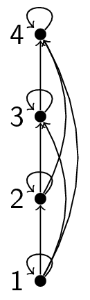
We now remove all self-loops:
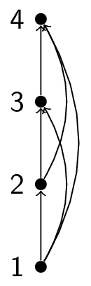
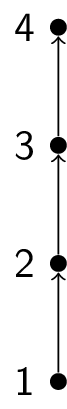
We now remove the arrows by placing all of the initial elements below the terminal elements:
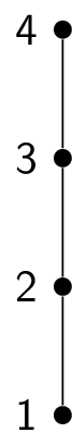
This is the Hasse diagram.
Here are some more examples of Hasse diagrams:
-
$(\{1,2,3,4,6,8,12\},|)$

-
$(\mathcal{P}{\{a,b,c\}}, \subseteq)$
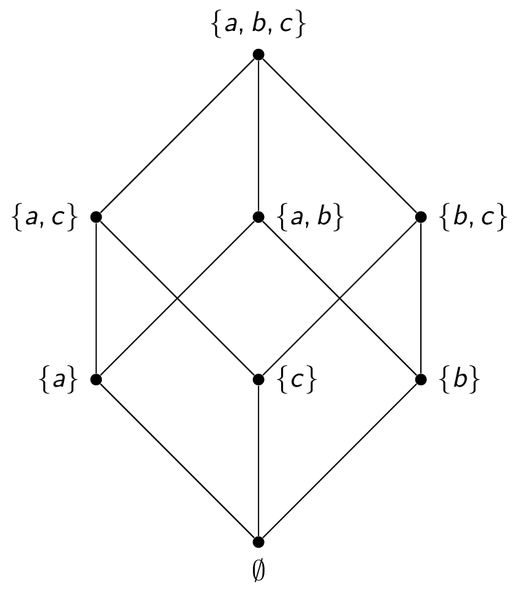
The other benefit of Hasse diagrams is that it is easier to pick out certain special elements.
An element $a$ is maximal in a poset $(S,\preceq)$ if there is no $b \in S$ with $a \prec b$ (that is, $a \preceq b$ but $a \neq b$).
An element $a$ is minimal in a poset $(S,\preceq)$ if there is no $b \in S$ with $b \prec a$.
In a Hasse diagram, the maximal element(s) are at the top and the minimal element(s) are at the bottom, but only in the sense of where the edges enter and leave, not their location on the diagram!
- $(\{1,2,3,4,6,8,12\},|)$: $8,12$ are maximal, $1$ is minimal
- $(\mathcal{P}{\{a,b,c\}}, \subseteq)$: $\{a,b,c\}$ is maximal, $\emptyset$ is minimal
Sometimes, there is an element greater than every other element. If $b \preceq a$ for all $b \in S$, then $a$ is the greatest element of $(S,\preceq)$. If $a \preceq b$ for all $b \in S$, then $a$ is the least element of $(S,\preceq)$. Both the greatest and least elements are unique when they exist.
- $(\{1,2,3,4,6,8,12\},|)$: $1$ is the least element, but there is no greatest element
- $(\mathcal{P}{\{a,b,c\}}, \subseteq)$: $\{a,b,c\}$ is the greatest element, $\emptyset$ is the least element
You might want to bound some subset of the poset. Given a poset $(S,\preceq)$ and a subset $A \subseteq S$:
- if $u \in S$ and $a \preceq u$ for all $a \in A$, then $u$ is a upper bound of $A$
- if $l \in S$ and $l \preceq a$ for all $a \in A$, then $l$ is a lower bound of $A$
For example:
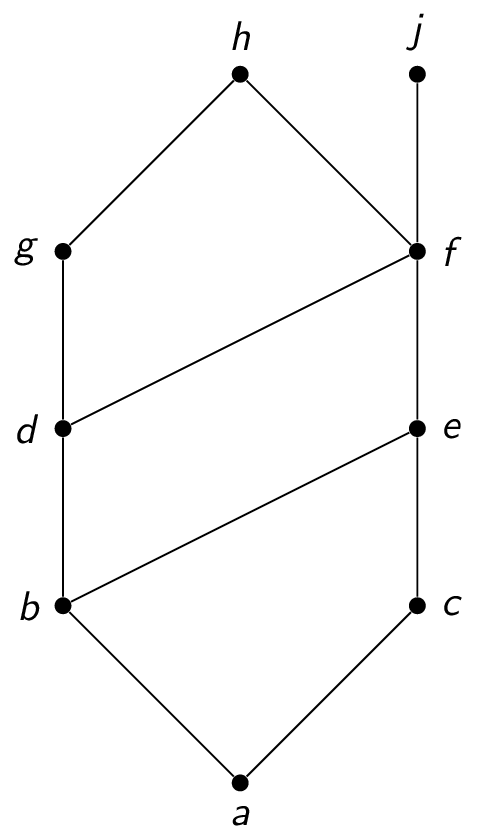
- upper bounds of $\{a,b,c\}$: $e,f,j,h$
- lower bounds of $\{a,b,c\}$: $a$
- upper bounds of $\{j,h\}$: none
- lower bounds of $\{j,h\}$: $a,b,c,d,e,f$
- upper bounds of $\{a,c,d,f\}$: $f,h,j$
- lower bounds of $\{a,c,d,f\}$: $a$
If $a \preceq x$ for any $a \in A$ and $x \preceq z$ for any upper bound $z$ of $A$ then $a$ is the least upper bound of $A$.
If $y$ is a lower bound of $A$ and $z \preceq y$ whenever $z$ is a lower bound of $A$ then $y$ is the greatest lower bound of $A$.
If the least upper bound or greatest lower bound exist, then they are unique.
In the previous example:
- the upper bounds of $\{b,d,g\}$ are $g,h$ and the least upper bound is $g$
- the lower bounds of $\{b,d,g\}$ are $a,b$ and the greatest lower bound is $b$
Topological Sorting
Suppose you are building a house. We can define a partial order on the "must be done before" relation: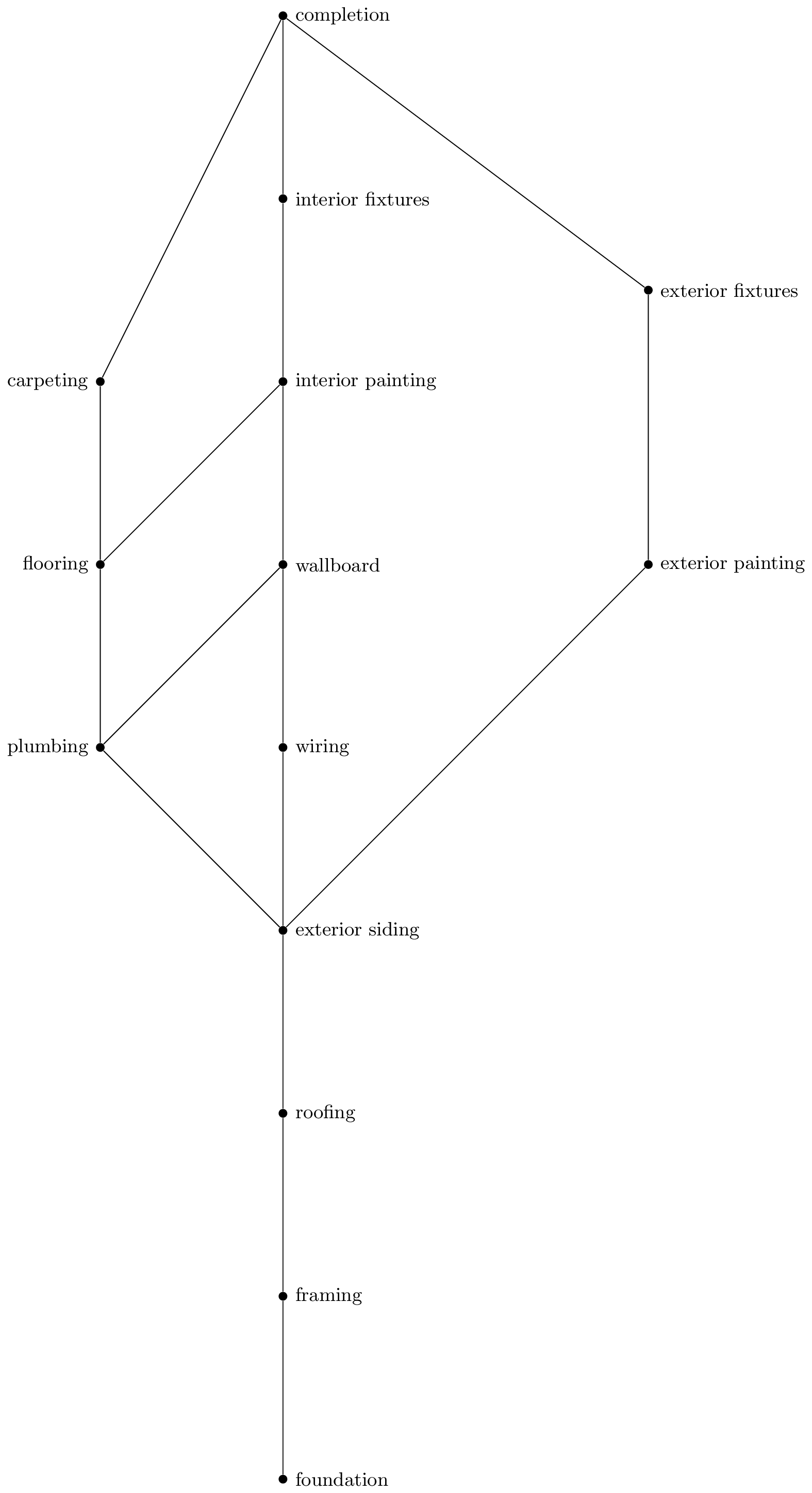
This is a partial order and must be respected when constructing a house. But this does not specify a valid ordering. There could be many! For example, we don't care if we do exterior painting or plumbing first (since they are incomparable elements).
We need a total order that respects the partial order. A total ordering $\preceq$ is compatible with a partial ordering $R$ if $a \preceq b$ whenever $aRb$.
Observe that every finite, non-empty poset has at least one minimal element.
Therefore, to find a compatible ordering, remove a minimal element and place it at the front of the total order. Now the initial partial order is a partial order with one fewer element. Keep doing this until all elements are gone. This is called topological sorting.
Here is how to topologically sort the poset $(\{1,2,3,4,6,8,12\},|)$. Here is the initial Hasse diagram:
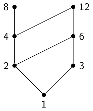
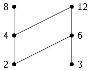
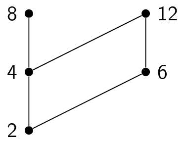
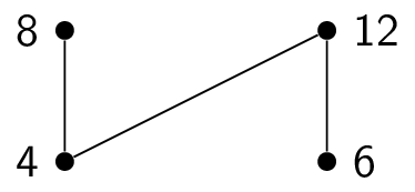
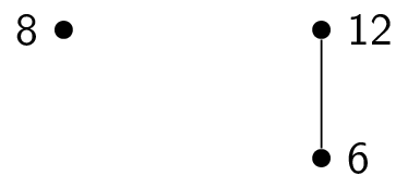
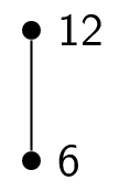

This means that the final element in the total order is $12$, giving us a total order of $1,3,2,4,8,6,12$. Other answers are possible!
A total order for house construction would be (for example) foundation, framing, roofing, exterior siding, plumbing, wiring, exterior painting, exterior fixtures, wallboard, flooring, interior painting, carpeting, interior fixtures, completion.
Graphs
Graphs can be used to model problems from virtually any field.
A graph is a pair $(V,E)$ where $V$ is a set called the vertex set and $E$ is a set called the edge set. Each edge in $E$ describes how vertices in $V$ are connected.
Here is an example of a graph:
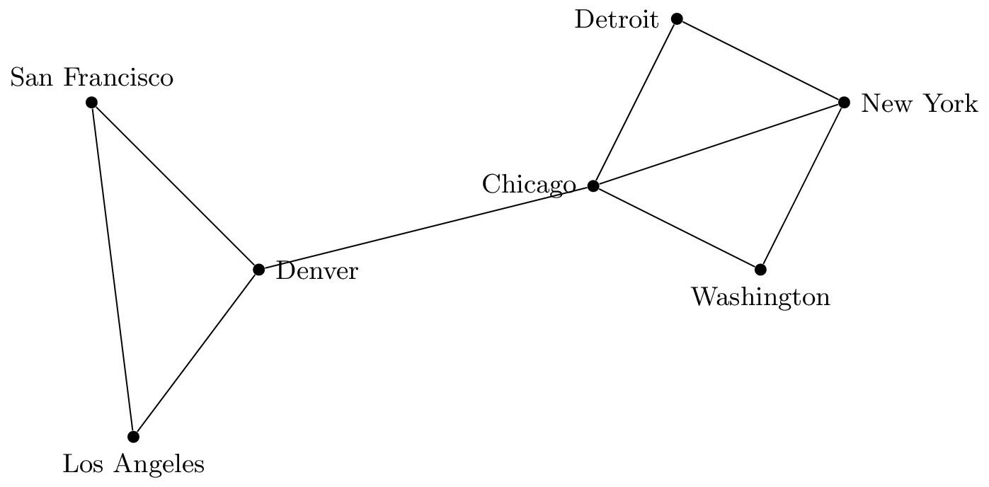
This particular graph is a simple graph:
- no edge connects a vertex to itself
- only one edge between two vertices
In this graph, edges don't have a direction. We say that the graph is undirected. Therefore, edges can be represented as sets consisting of two vertices. For the above graph,
- $V = \{ \text{San Francisco}, \text{Los Angeles}, \text{Denver}, \text{Chicago}, \text{Detroit}, \text{New York}, \text{Washington} \}$
- $E = \{\\ \,\;\{ \text{San Francisco}, \text{Denver} \},\\ \;\{ \text{San Francisco}, \text{Los Angeles} \},\\ \;\{ \text{Los Angeles}, \text{Denver} \},\\ \;\{ \text{Denver}, \text{Chicago} \},\\ \;\{ \text{Chicago}, \text{Detroit} \},\\ \;\{ \text{Detroit}, \text{New York} \},\\ \;\{ \text{New York}, \text{Washington} \},\\ \;\{ \text{Washington}, \text{Chicago} \},\\ \;\{ \text{Chicago}, \text{New York} \}\\ \}$
Sometimes, we might want to allow multiple edges between vertices. Such graphs are called multigraphs:
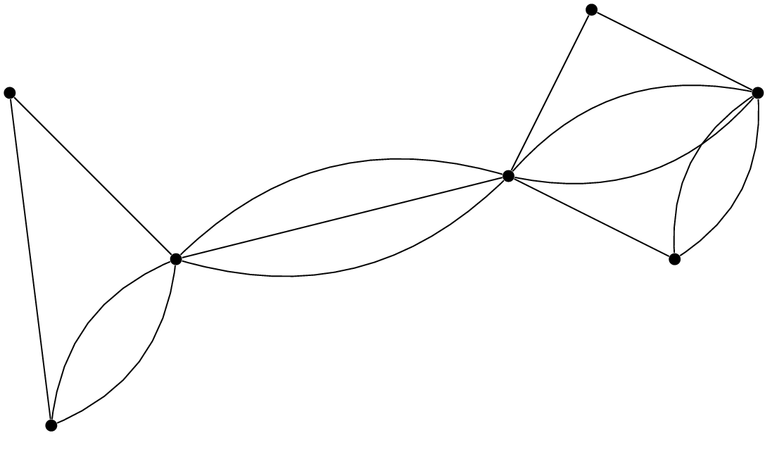
Edges are still undirected; we can represent them as sets of two vertices. However, now these sets can appear more than once. We say that if there are $m$ distinct edges between $u$ and $v$, the edge $\{u,v\}$ has multiplicity $m$. Multigraphs are used, for example, to model redundant connections in a network.
We might also want to relax the restriction that there are no edges between a vertex and itself. Such edges are called self-loops and a graph that contains self-loops is called a pseudograph. Self-loops model such things as loopbacks in networks.
We can also have directed versions of these graphs, where edges only go in one direction. Here is an example of a directed multigraph:
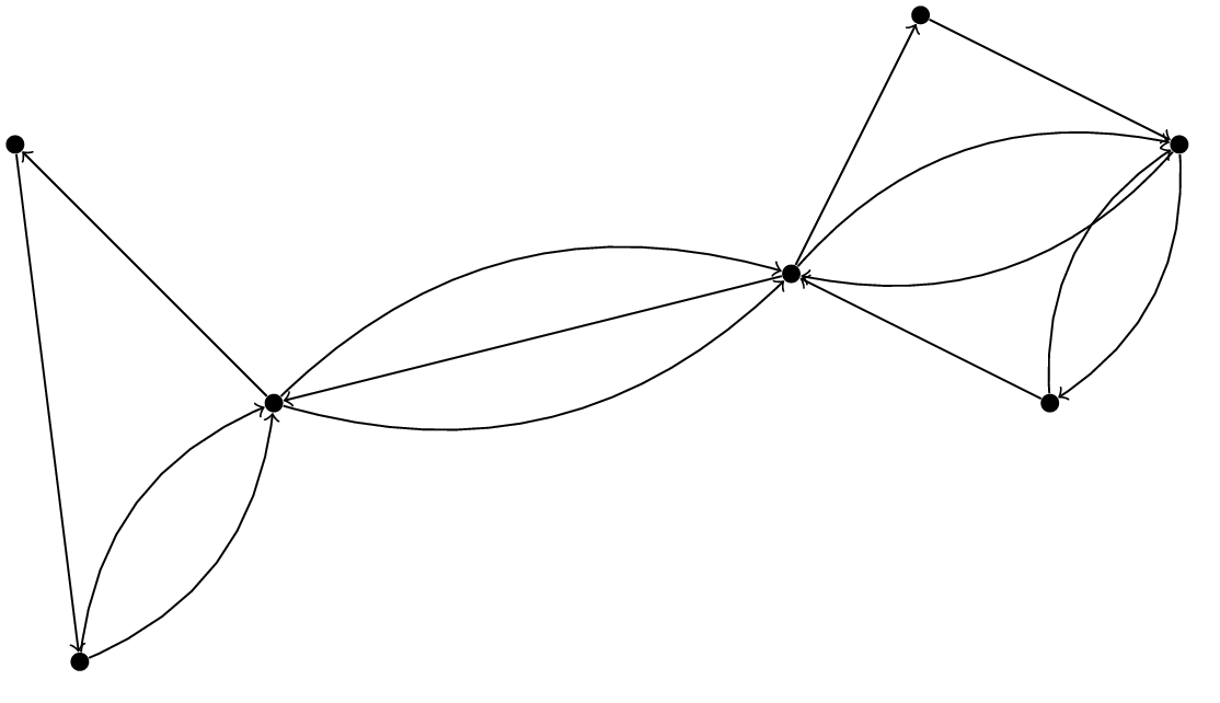
Directed edges can be represented as an ordered pair $(u,v)$ instead of a set $\{u,v\}$. Directed edges model such things as single duplex lines or one-way streets in road networks.
There are many uses of graphs:
- social networks (Facebook, etc.)
- Hollywood graph (Six Degrees of Kevin Bacon)
- Web graph
Representing Graphs
We need a way of representing graphs if we want to perform operations on them. We could simply list the vertices and edges, but that is a lot of work and it is hard to extract much information from that representation.
Here are two alternatives:
-
adjacency list: For each vertex, list the vertices that are connected to that vertex by an edge. Such vertices are said to be adjacent. (This works for both directed and undirected graphs, even if they contain loops.)
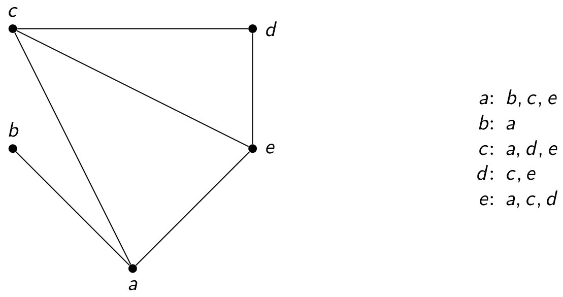
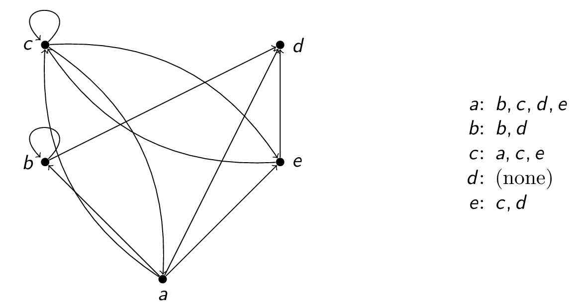
-
adjacency matrix: one row and one column for each vertex $v_1,v_2,\ldots,v_n$, row $i$ column $j$ is $1$ if the edge is in $E$, $0$ otherwise. (For this to work, you have to fix some ordering on the vertices.)
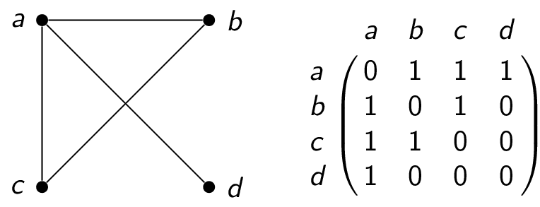
For simple undirected graphs, the adjacency matrix is symmetric ($a_{ij} = a_{ji}$ and the main diagonal is all $0$s ($a_{ii} = 0$) since no self-loops are allowed.
In general, we can allow for multigraphs by using the multiplicities as entries instead of just $0$ or $1$.
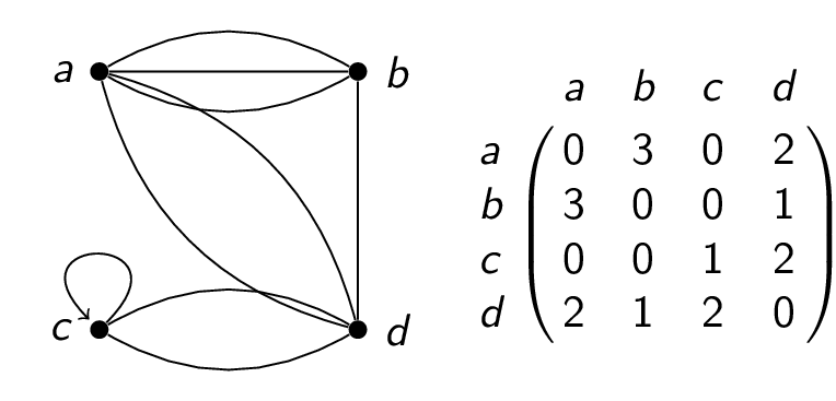
Adjacency and Degree
Let $G = (V,E)$ be a graph.
- two vertices are adjacent (are neighbours) in $G$ if $u$ and $v$ are endpoints of some edge in $G$
- if edge $e$ connects $u$ and $v$, we say $e$ is incident on $u$ (and $v$) or incident with $u$ and $v$
- the degree of a vertex in an undirected graph is the number of edges incident with it, denoted by $\deg{v}$. If a self-loop is present, it is counted twice!
For example:
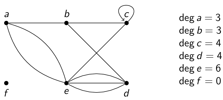
The Handshaking Theorem says that, for a graph $G=(V,E)$, we always have $$\sum_{v \in V} \deg(v) = 2|E|$$
For a directed edge $(u,v)$ in a directed graph, $u$ is the initial vertex and $v$ is the terminal vertex or end vertex.
- the number of incoming edges to $v$ (that is, the number of edges with $v$ as terminal) is denoted $\deg^-(v)$ and called the in-degree of $v$
- the number of outgoing edges from $u$ (that is, the number of edges with $u$ as initial) is denoted $\deg^+(u$ and called the out-degree of $u$
Note that $\sum_{v \in V} \deg^-(v) = \sum_{v \in V} \deg^+(v) = |E|$.
Some Special Graphs
There are a few (types of) graphs with special names:
-
the complete graph on $n$ vertices, $K_n$, has $n$ vertices, each of which is connected to all other vertices. From left to right, we have $K_1, K_2, K_3, K_4, K_5$:
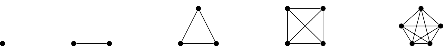
-
the cycle on $n \ge 3$ vertices, $C_n$, has vertices $v_1,v_2,\ldots,v_n$ and edges $\{v_1,v_2\},\{v_2,v_3\},\ldots,\{v_{n-1},v_n\},\{v_n,v_1\}$. From left to right, we have $C_3, C_4, C_5$:
-
the wheel on $n \ge 3$ vertices, $W_n$, takes $C_n$ and adds one vertex connected to all the other vertices. From left to right, we have $W_3,W_4,W_5$:
-
a bipartite graph $G=(V,E)$ partitions $V$ into $V_1$ and $V_2$ such that $V_1 \cup V_2 = V$ and $V_1 \cap V_2 = \emptyset$, and every edge in $E$ has one endpoint in $V_1$ and one endpoint in $V_2$. This is the same as assigning one of two colours to every vertex such that no adjacent vertices have the same colour. The complete bipartite graph $K_{m,n}$ has partitions of size $m$ and $n$ and every element in one partition is connected to every element of the other partition. Here are $K_{2,3}$ and $K_{3,3}$:
Subgraphs
A subgraph of a graph $G=(V,E)$ is a graph $H=(W,F)$ such that $W \subseteq V$ and $F \subseteq E$. A subgraph $H$ of $G$ is a proper subgraph of $G$ if $H \neq G$.
For example, on the left we have $K_5$ and on the right is a subgraph of $K_5$.
A subgraph is spanning if it contains all vertices of the original graph.
Connectivity
Sometimes, we want to know if two vertices in a graph are connected by a sequence of edges that might visit other vertices on the way (for example, can two computers on a network communicate?)
A path is a sequence of edges that begins at a vertex and travels from vertex to vertex along edges of the graph.
More formally, a path of length $n \ge 0$ from vertex $u$ to vertex $v$ in $G$ is a sequence of $n$ edges $e_1,e_2,\ldots,e_n$ of $G$ such that $e_1 = \{ x_0 = u, x_1 \}, e_2 = \{ x_1,x_2 \}, \ldots, e_n = \{x_{n-1},x_n\}$.
- if the graph is simple, we can just use the vertex sequence to label the path
- the path is a circuit if $u=v$
- the path passes through vertices $x_1,x_2,\ldots,x_{n-1}$ and traverses edges $e_1,e_2,\ldots,e_n$
- a path is simple if it does not traverse an edge more than once
For example:
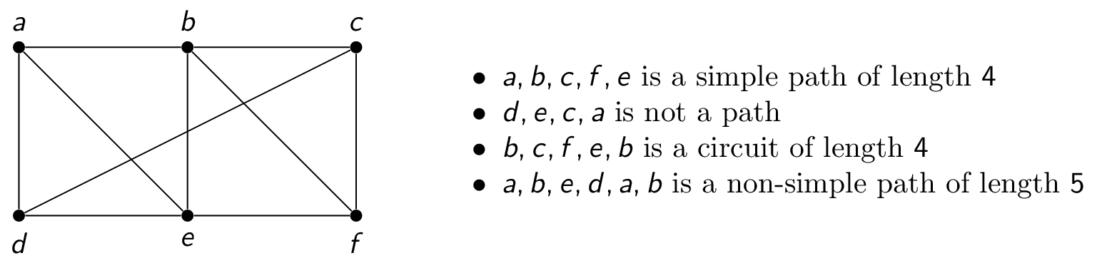
An undirected graph is connected if there is a path between every two distinct vertices in the graph. For example, the graph on the left is connected but the graph on the right is disconnected.
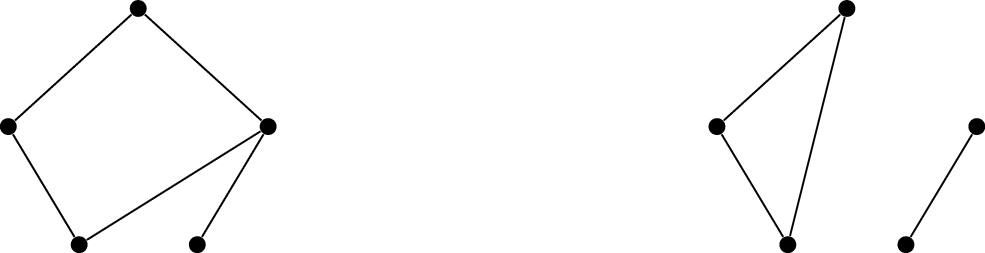
The different parts that are maximally connected are called connected components.
One special type of connected (sub)graph is a tree, which is a connected undirected graph with no simple circuits. For example, the graph on the left is a tree; the graph in the center is not a tree because it contains a circuit; and the graph on the right is not a tree because it is not connected.
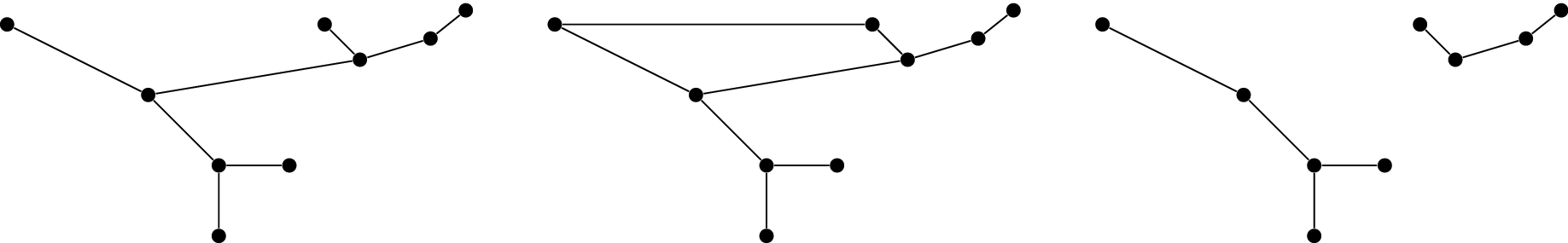
Because trees are "simple" in structure, we often want to find a spanning subgraph that is a tree:
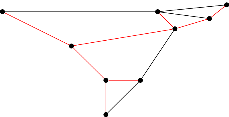
In the graph above, the red edges form a spanning subgraph because every vertex appears exactly once. It is a tree because it is connected and contains no circuits.
Returning to subgraphs in general, we note that sometimes removing a single vertex or edge would cause a graph to become disconnected:
- a cut vertex is a vertex whose removal disconnects the remaining graph (note that any edges incident on the removed vertex are removed too)
- a cut edge is an edge whose removal disconnects the remaining graph
For example, consider the following graph:
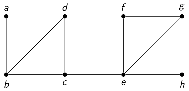
The cut vertices are $b,c,e$, and the cut edges are $\{a,b\},\{c,e\}$.
We can also talk about connectivity in directed graphs:- a directed graph is strongly connected if there is a path from $a$ to $b$ and from $b$ to $a$ for every pair of vertices $a$ and $b$
- a directed graph is weakly connected if the graph is connected when you ignore the directions of the edges (that is, the "underlying undirected graph")
For example, the graph on the left is both strongly and weakly connected, while the graph on the right is only weakly connected since there is no path from $a$ to $b$.
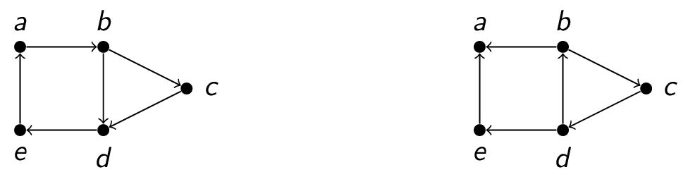
Depth First Search
Suppose you are trying to explore a graph:
- see what computers are connected to a network
- visit cities connected by flights
- $\ldots$
How do you do this in an orderly way, so that you don't end up getting lost (looping forever)? Idea:
- mark all vertices as unvisited
- start at an arbitrary vertex
- go to an unvisited neighbour
- repeat until you have seen all unvisited neighbours
- go back
This approach is called a depth first search. Consider the following graph:
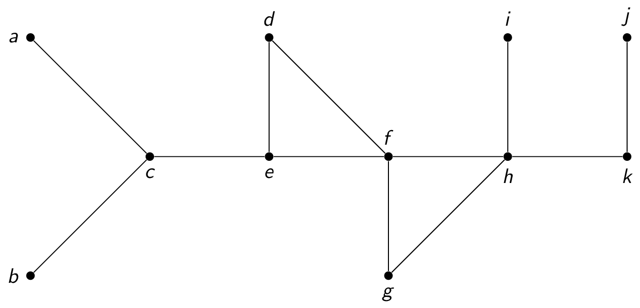
A depth first search proceeds as follows:
- start at (for example) $f$
- visit $f,g,h,k,j$
- backtrack to $k$
- backtrack to $h$
- visit $i$
- backtrack to $h$
- backtrack to $f$
- visit $f,d,e,c,a$
- backtrack to $c$
- visit $c,b$
Notice that this produces a spanning tree, since all nodes are visited and there are no cycles (since having a cycle would mean visiting an already-visited node).
Depth first search has many applications. For example:
- find paths, circuits
- find connected components
- find cut vertices
- many AI applications
Breadth First Search
Instead of always going as deep as possible (as in depth first search), we can try to explore gradually at specific distances from the starting vertex. Such a search is called a breadth first search and proceeds as follows:
- keep a list of vertices seen so far, initially containing an arbitrary vertex
- add all adjacent vertices to the end of the list
- take the first vertex off the list and visit it
- add its unvisited neighbours to the end of the list
- repeat previous two steps until list is empty
Consider the following graph:
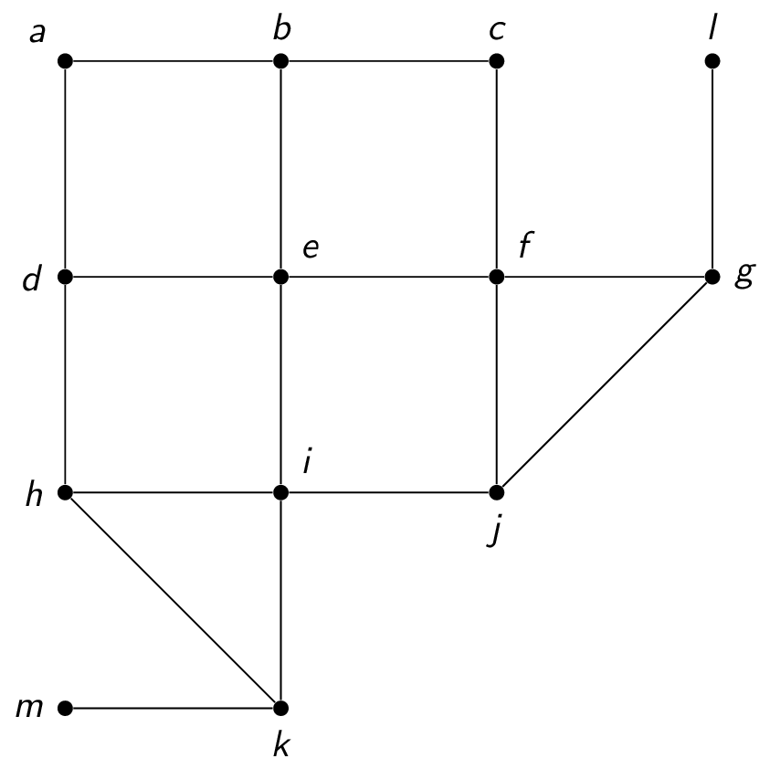
A breadth first search proceeds as follows:
- start at (for example) $e$
- visit $b,d,f,i$ (the vertices at distance $1$ from $e$)
- visit $a,c,h,j,g,k$ (the vertices at distance $2$ from $e$)
- visit $l,m$ (the vertices at distance $3$ from $e$)
The process also produces a spanning tree. In fact, this also gives the path with the fewest edges from the start node to any other node. This is the same as the shortest path if all edges are the same length or have the same cost.
Planarity
Sometimes, it is easy to get confused about a graph when looking at a picture of it because many of the edges cross and it is difficult to determine what edge is going where. It is often nicer to look at graphs whose edges do not cross.
Notice that there are often many ways to draw the same graph. For example, here are two ways of visualizing the complete graph $K_4$:
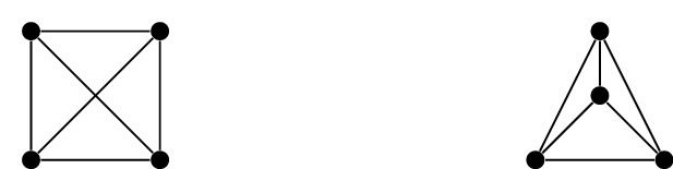
Even though they are drawn differently, they are essentially the same graph: four vertices where each vertex is connected to every other vertex. However, the drawing on the right is "nicer" because none of its edges cross.
We call a graph planar if it is possible to draw it in the plane without any edges crossing. Such a drawing is called a planar representation of the graph.
The above example shows that $K_4$ is planar.
Not all graphs are planar, however! For example, $K_{3,3}$ cannot be drawn without crossing edges. To see this, recall what $K_{3,3}$ looks like:
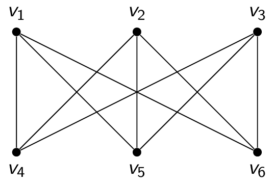
Observe that the vertices $v_1$ and $v_2$ must be connected to both $v_4$ and $v_5$. These four edges form a closed curve that splits the plane into two regions $R_1$ and $R_2$. The vertex $v_3$ is either inside the region $R_1$ or $R_2$. Let's suppose that $v_3$ is in $R_2$ for the time being. Since $v_3$ is connected to $v_4$ and $v_5$, it divides $R_2$ into two subregions, $R_{21}$ and $R_{22}$. The situation is as follows:
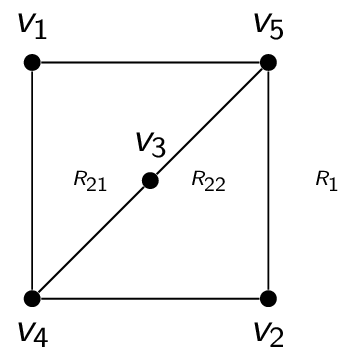
Now, consider where to place the final vertex $v_6$. If it is placed in $R_1$, then the edge between $v_3$ and $v_6$ must have a crossing. If it is placed in $R_{21}$, then the edge between $v_2$ and $v_6$ must have a crossing. If it is placed in $R_{22}$, then the edge between $v_1$ and $v_6$ must have a crossing. A similar argument works for the case when $v_6$ is in $R_2$.
We have shown that $K_{3,3}$ is not planar: it cannot be drawn without crossings.
Properties of Planar Graphs
Planar graphs have some nice properties.
Let $G=(V,E)$ be a planar graph, and let $v$ denote the number of vertices, $e$ denote the number of edges, and $f$ denote the number of faces (including the "outer face"). Then $v - e + f = 2$. This is known as Euler's formula.
To prove this, consider two cases. If $G$ is a tree, then it must be the case that $e=v-1$ and $f=1$ (since otherwise there would be a cycle). Therefore, $v - e + f = v - (v-1) + 1 = v-v+1+1 = 2$. Otherwise, if $G$ is not a tree, then $G$ must have a cycle with at least $3$ edges. If we delete an edge on that cycle, $v$ stays the same, while $e$ and $f$ both decrease by $1$ and so the equality is still true. (This is a proof by induction in diguise!)
Another nice property is that if $G=(V,E)$ is a connected planar simple graph and $|V| \ge 3$, then $|E| \le 3|V|-6$. This is a consequence of Euler's formula. This property can be used to prove that $K_5$ is not planar. To see this, observe that $K_5$ has five vertices and ten edges; this does not satisfy $|E| \le 3|V|-6$ and therefore the $K_5$ cannot be planar.
If $G=(V,E)$ is a connected planar simple graph, then $G$ has a vertex of degree at most $5$. To see this, observe that if $G$ has one or two vertices, the result is true. If $G$ has at least three vertices, we know that $|E| \le 3|V|-6$, so $2|E| \le 6|V|-12$. The Handshaking Theorem says that $\sum_{v \in V} \deg{v} = 2|E|$. If the degree of every vertex were at least $6$, then we would have $2|E| \ge 6|V|$, which contradicts the inequality $2|E| \le 6|V|-12$.
Planar graphs also have small average degree. The average degree of a graph $G=(V,E)$ is $2|E|/|V|$. Using the fact that $|E| \le 3|V|-6$ (when $|V| \ge 3$), we get that $$\frac{2|E|}{|V|} \le \frac{2(3|V|-6)}{|V|} \le 6 - \frac{12}{|V|}$$ as long as $|V| \ge 3$, this is strictly less than $6$. This means that, on average, the degrees of vertices in a planar graph are small.
Graph Colouring
As mentioned earlier, many applications in the real world can be modelled as graphs. One recurring application is to colour a graph: assign a colour to every vertex so that no two adjacent vertices share the same colour.
Consider the graph of courses at Carleton where two courses are connected by an edge if there is at least one student in both courses. To schedule exams, each vertex will be assigned a colour to represent its time slot. To avoid conflicts, courses with common students must have their exams scheduled at different times: they must be assigned different colours.
A colouring of a simple graph is the assignment of a colour to each vertex of the graph such that no two adjacent vertices are assigned the same colour. The chromatic number of a graph is the smallest number of colours required to colour the graph, and is usually denoted $\chi(G)$ for a graph $G$. For example:
- the chromatic number of $K_n$ is $n$, since all pairs of vertices are adjacent
- the chromatic number of $K_{m,n}$ is $2$: colour one part of the partition one colour, and the other part of the partition the other colour. Since there are no edges within one part of the partition, there are no adjacent vertices with the same colour
- the chromatic number of $C_n$ is $2$ when $n$ is even and $3$ when $n$ is odd
One particularly interesting case is computing the chromatic number for simple planar graphs. Here is a proof that the chromatic number of a planar graph is at most $6$:
We will prove the statement by induction on the number of vertices.
- Basis step: Suppose we have a graph with $|V| \le 6$. Simply give each vertex a different colour.
- Inductive hypothesis: Assume that any simple planar graph on $n$ vertices can be coloured with at most $6$ colours for some arbitrary $n$.
- Inductive step: Let $G$ be any simple planar graph on $n+1$ vertices. We know that $G$ must have at least one vertex $v$ with degree at most $5$. Remove $v$ from $G$ to form a simple planar graph with $n$ vertices. By our inductive hypothesis, this graph can be coloured with at most $6$ colours. Now, add back in the vertex $v$. Since it had degree at most $5$, it has at most $5$ neighbours and therefore at most $5$ colours adjacent to it. This leaves at least one more colour for it.
Computing the chromatic number of a general graph is tricky! There are no efficient algorithms to determine $\chi(G)$ for a general graph $G$ if nothing else is known about it.
At least one colour and at most $n$ colours are required, so $1 \le \chi(G) \le n$ for any graph $G$. The only graphs that require only one colour are those without edges. The graphs that require two colours are bipartite graphs (including trees, for example).
What if we just want some colouring of $G$, perhaps using more than $\chi(G)$ colours? One possible algorithm is to use a greedy colouring. To do this, order the vertices in some specific way, and assign each vertex in sequence the smallest available colour not used by that vertex's neighbours. The trick is using a good order!
- There is always an order that results in $\chi(G)$ colours, but we don't know how to find it efficiently.
- There are really bad orders that use many more colours than necessary. For example, $K_{n,n}$ can be ordered by going through one partition and then the other and therefore use $2$ colours, or ordered by alternating one element from each partition and therefore use $n$ colours.
- One reasonable ordering of the vertices is by non-increasing degree. If the largest degree in the graph is $\Delta$, then at most $\Delta+1$ colours will be used.
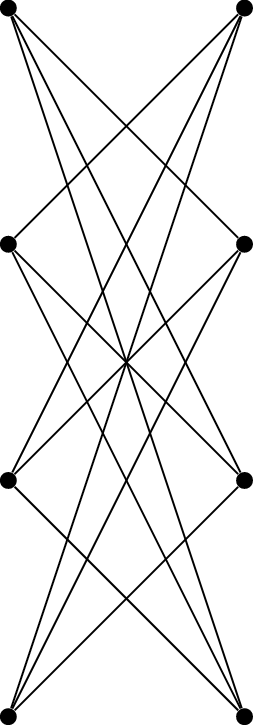
Consider the graph above. If the ordering alternates from left to right, a $4$-colouring is produced. If the ordering goes all the way up the left and then all the way up the right, a $2$-colouring is produced. This graph can be generalized to have $k$ vertices on the left and $k$ vertices on the right. The orderings would then produce a $k$-colouring and a $2$-colouring, respectively. This is a huge difference!