Depth First Search
Suppose you are trying to explore a graph:
- see what computers are connected to a network
- visit cities connected by flights
- $\ldots$
How do you do this in an orderly way, so that you don't end up getting lost (looping forever)? Idea:
- mark all vertices as unvisited
- start at an arbitrary vertex
- go to an unvisited neighbour
- repeat until you have seen all unvisited neighbours
- go back
This approach is called a depth first search. Consider the following graph:
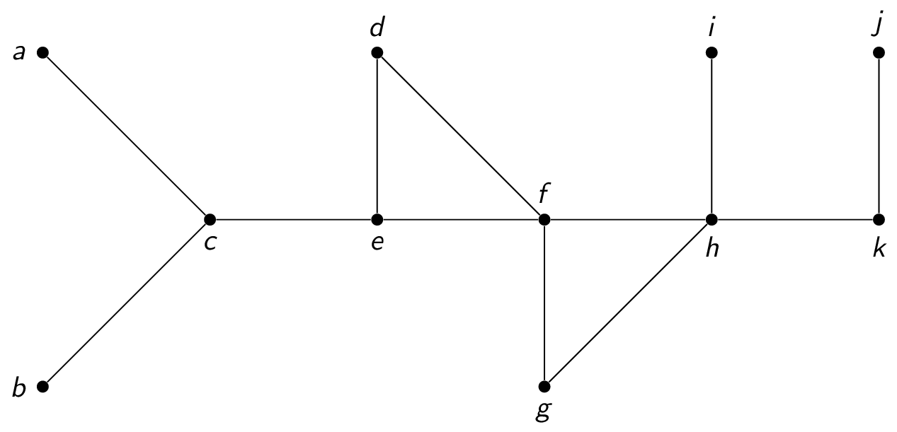
A depth first search proceeds as follows:
- start at (for example) $f$
- visit $f,g,h,k,j$
- backtrack to $k$
- backtrack to $h$
- visit $i$
- backtrack to $h$
- backtrack to $f$
- visit $f,d,e,c,a$
- backtrack to $c$
- visit $c,b$
Notice that this produces a spanning tree, since all nodes are visited and there are no cycles (since having a cycle would mean visiting an already-visited node).
Depth first search has many applications. For example:
- find paths, circuits
- find connected components
- find cut vertices
- many AI applications
Breadth First Search
Instead of always going as deep as possible (as in depth first search), we can try to explore gradually at specific distances from the starting vertex. Such a search is called a breadth first search and proceeds as follows:
- keep a list of vertices seen so far, initially containing an arbitrary vertex
- add all adjacent vertices to the end of the list
- take the first vertex off the list and visit it
- add its unvisited neighbours to the end of the list
- repeat previous two steps until list is empty
Consider the following graph:
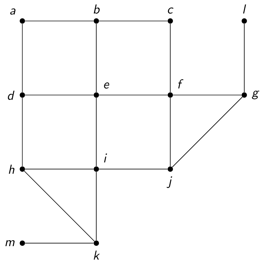
A breadth first search proceeds as follows:
- start at (for example) $e$
- visit $b,d,f,i$ (the vertices at distance $1$ from $e$)
- visit $a,c,h,j,g,k$ (the vertices at distance $2$ from $e$)
- visit $l,m$ (the vertices at distance $3$ from $e$)
The process also produces a spanning tree. In fact, this also gives the path with the fewest edges from the start node to any other node. This is the same as the shortest path if all edges are the same length or have the same cost.
Planarity
Sometimes, it is easy to get confused about a graph when looking at a picture of it because many of the edges cross and it is difficult to determine what edge is going where. It is often nicer to look at graphs whose edges do not cross.
Notice that there are often many ways to draw the same graph. For example, here are two ways of visualizing the complete graph $K_4$:
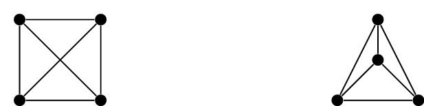
Even though they are drawn differently, they are essentially the same graph: four vertices where each vertex is connected to every other vertex. However, the drawing on the right is "nicer" because none of its edges cross.
We call a graph planar if it is possible to draw it in the plane without any edges crossing. Such a drawing is called a planar representation of the graph.
The above example shows that $K_4$ is planar.
Not all graphs are planar, however! For example, $K_{3,3}$ cannot be drawn without crossing edges. To see this, recall what $K_{3,3}$ looks like:
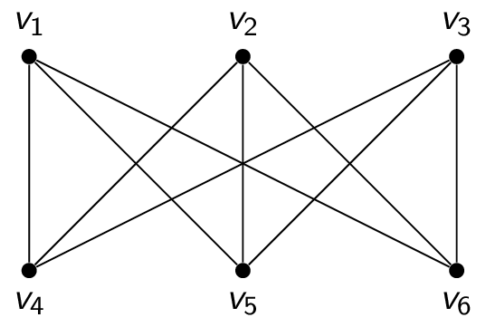
Observe that the vertices $v_1$ and $v_2$ must be connected to both $v_4$ and $v_5$. These four edges form a closed curve that splits the plane into two regions $R_1$ and $R_2$. The vertex $v_3$ is either inside the region $R_1$ or $R_2$. Let's suppose that $v_3$ is in $R_2$ for the time being. Since $v_3$ is connected to $v_4$ and $v_5$, it divides $R_2$ into two subregions, $R_{21}$ and $R_{22}$. The situation is as follows:
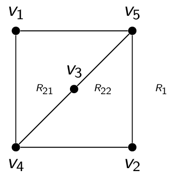
Now, consider where to place the final vertex $v_6$. If it is placed in $R_1$, then the edge between $v_3$ and $v_6$ must have a crossing. If it is placed in $R_{21}$, then the edge between $v_2$ and $v_6$ must have a crossing. If it is placed in $R_{22}$, then the edge between $v_1$ and $v_6$ must have a crossing. A similar argument works for the case when $v_6$ is in $R_2$.
We have shown that $K_{3,3}$ is not planar: it cannot be drawn without crossings.
Properties of Planar Graphs
Planar graphs have some nice properties.
Let $G=(V,E)$ be a planar graph, and let $v$ denote the number of vertices, $e$ denote the number of edges, and $f$ denote the number of faces (including the "outer face"). Then $v - e + f = 2$. This is known as Euler's formula.
To prove this, consider two cases. If $G$ is a tree, then it must be the case that $e=v-1$ and $f=1$ (since otherwise there would be a cycle). Therefore, $v - e + f = v - (v-1) + 1 = v-v+1+1 = 2$. Otherwise, if $G$ is not a tree, then $G$ must have a cycle with at least $3$ edges. If we delete an edge on that cycle, $v$ stays the same, while $e$ and $f$ both decrease by $1$ and so the equality is still true. (This is a proof by induction in diguise!)
Another nice property is that if $G=(V,E)$ is a connected planar simple graph and $|V| \ge 3$, then $|E| \le 3|V|-6$. This is a consequence of Euler's formula. This property can be used to prove that $K_5$ is not planar. To see this, observe that $K_5$ has five vertices and ten edges; this does not satisfy $|E| \le 3|V|-6$ and therefore the $K_5$ cannot be planar.
If $G=(V,E)$ is a connected planar simple graph, then $G$ has a vertex of degree at most $5$. To see this, observe that if $G$ has one or two vertices, the result is true. If $G$ has at least three vertices, we know that $|E| \le 3|V|-6$, so $2|E| \le 6|V|-12$. The Handshaking Theorem says that $\sum_{v \in V} \deg{v} = 2|E|$. If the degree of every vertex were at least $6$, then we would have $2|E| \ge 6|V|$, which contradicts the inequality $2|E| \le 6|V|-12$.
Planar graphs also have small average degree. The average degree of a graph $G=(V,E)$ is $2|E|/|V|$. Using the fact that $|E| \le 3|V|-6$ (when $|V| \ge 3$), we get that $$\frac{2|E|}{|V|} \le \frac{2(3|V|-6)}{|V|} \le 6 - \frac{12}{|V|}$$ as long as $|V| \ge 3$, this is strictly less than $6$. This means that, on average, the degrees of vertices in a planar graph are small.
Graph Colouring
As mentioned earlier, many applications in the real world can be modelled as graphs. One recurring application is to colour a graph: assign a colour to every vertex so that no two adjacent vertices share the same colour.
Consider the graph of courses at Carleton where two courses are connected by an edge if there is at least one student in both courses. To schedule exams, each vertex will be assigned a colour to represent its time slot. To avoid conflicts, courses with common students must have their exams scheduled at different times: they must be assigned different colours.
A colouring of a simple graph is the assignment of a colour to each vertex of the graph such that no two adjacent vertices are assigned the same colour. The chromatic number of a graph is the smallest number of colours required to colour the graph, and is usually denoted $\chi(G)$ for a graph $G$. For example:
- the chromatic number of $K_n$ is $n$, since all pairs of vertices are adjacent
- the chromatic number of $K_{m,n}$ is $2$: colour one part of the partition one colour, and the other part of the partition the other colour. Since there are no edges within one part of the partition, there are no adjacent vertices with the same colour
- the chromatic number of $C_n$ is $2$ when $n$ is even and $3$ when $n$ is odd
One particularly interesting case is computing the chromatic number for simple planar graphs. Here is a proof that the chromatic number of a planar graph is at most $6$:
We will prove the statement by induction on the number of vertices.
- Basis step: Suppose we have a graph with $|V| \le 6$. Simply give each vertex a different colour.
- Inductive hypothesis: Assume that any simple planar graph on $n$ vertices can be coloured with at most $6$ colours for some arbitrary $n$.
- Inductive step: Let $G$ be any simple planar graph on $n+1$ vertices. We know that $G$ must have at least one vertex $v$ with degree at most $5$. Remove $v$ from $G$ to form a simple planar graph with $n$ vertices. By our inductive hypothesis, this graph can be coloured with at most $6$ colours. Now, add back in the vertex $v$. Since it had degree at most $5$, it has at most $5$ neighbours and therefore at most $5$ colours adjacent to it. This leaves at least one more colour for it.
Computing the chromatic number of a general graph is tricky! There are no efficient algorithms to determine $\chi(G)$ for a general graph $G$ if nothing else is known about it.
At least one colour and at most $n$ colours are required, so $1 \le \chi(G) \le n$ for any graph $G$. The only graphs that require only one colour are those without edges. The graphs that require two colours are bipartite graphs (including trees, for example).
What if we just want some colouring of $G$, perhaps using more than $\chi(G)$ colours? One possible algorithm is to use a greedy colouring. To do this, order the vertices in some specific way, and assign each vertex in sequence the smallest available colour not used by that vertex's neighbours. The trick is using a good order!
- There is always an order that results in $\chi(G)$ colours, but we don't know how to find it efficiently.
- There are really bad orders that use many more colours than necessary. For example, $K_{n,n}$ can be ordered by going through one partition and then the other and therefore use $2$ colours, or ordered by alternating one element from each partition and therefore use $n$ colours.
- One reasonable ordering of the vertices is by non-increasing degree. If the largest degree in the graph is $\Delta$, then at most $\Delta+1$ colours will be used.
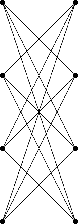
Consider the graph above. If the ordering alternates from left to right, a $4$-colouring is produced. If the ordering goes all the way up the left and then all the way up the right, a $2$-colouring is produced. This graph can be generalized to have $k$ vertices on the left and $k$ vertices on the right. The orderings would then produce a $k$-colouring and a $2$-colouring, respectively. This is a huge difference!