Planar Point Location

Randomized Incremental Method

The presentation of the Randomized incremental method here follows the treatment in de Berg (2000) which is itself based on Siedel (1991). To begin the description of the algorithm we will first review the two data structures involved, the trapezoid map, T and its associated search structure D.

The Trapezoid Map

Figure 1 shows a simple trapezoidal map generated by three segments, s₁, s₂, and s₃. The map is linked together through the adjacency of its constituent trapezoids. The map includes a set of records recording each line segment in the input subdivision S and the endpoints of these segments. These records serve as the leftp(t), rightp(t), top(t), and bottom(t) for each trapezoid, which holds pointers to these records. In addition each trapezoid stores pointers to its, up to four, neighbouring trapezoids. Note that geometry for a trapezoid need to be directly stored as it can be obtained from leftp(t), rightp(t), top(t), and bottom(t) in constant time.

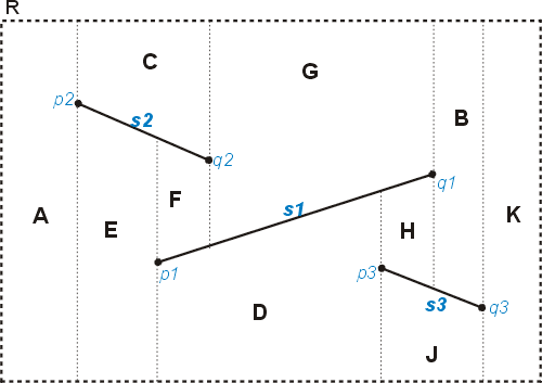
Fig. 1: A trapezoidal map generated by three segments s1, s2, and s3 (based on de Berg (2000)).

The Search Structure

The search structure associated with the trapezoid map in figure 1 is given in figure 2 below. The search structure is a fundamental part of the trapezoid construction algorithm, and is a directed acyclic graph. The structure has the trapezoids as the leafs of the structure, and two types of internal nodes, x-nodes and y-nodes. An x-nodes stores a segment endpoint that defines a vertical extension in the trapezoid map, and has leftChild() and rightChild() pointers to nodes. A y-node stores a line segment and its children are also recorded by the pointers are aboveChild() and belowChild() depending on whether the child item is above or below the segment stored at the y-node. The query procedure is quite simple and psuedo-code for a recursive implementation is given below figure 2.

The two structures are very closely linked, as each leaf in D containes a pointer to its associated trapezoid in trapezoid map T, likewise the trapezoid map trapezoids store pointers to their corresponding leaf nodes in D.

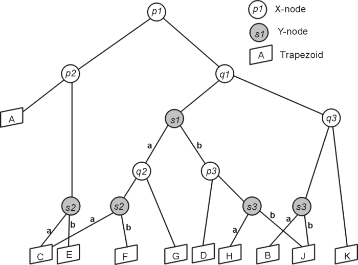
Fig. 2: Resulting search structure for trapezoid map in Fig 1. For x-nodes the left and right child shown by the pointer directions, for above and below children of y-nodes the pointer type has been indicated by the letter a(bove) or b(elow) (based on de Berg (2000))..

Algorithm QueryTrapezoidMap( D, n, p)
Input: T is the trapezoid map search structure, n is a 
   node in the search structure and p is a query point.
Output:  A pointer to the node in D for the trapezoid 
   containing the point p.
1. if ( n is a Trapezoid Node)
	return n;
2. if ( n is an X-node)
  a. if the x-coordinate of p the is less than the x-coordinate 
    of the point stored at this node then 
		return QueryTrapezoidMap(T, leftChild(n), p).
	else 
		return QueryTrapezoidMap(T, rightChild(n), p)
3. if (n is a Y-node)
  a. if p is above the segment stored at n then
		return QueryTrapezoidMap(T, aboveChild(n), p).
	 else 
	 	return QueryTrapezoidMap(T, belowChild(n), p)

Note that D is not necessarily balanced, and thus for a unfavourable set of segment insertions the structure can degraded and lead to poor query performance. By inserting segments in random order the resulting structure is well-balanced and can be expected to have good query behaviour. The psuedo-code listed below as BuildTrapezoidMap lists at a high level the steps required to update the two search structures following a segment insertion.

Algorithm BuildTrapezoidalMap( S )
Input: S is the set of line segments forming a planar subdivision.
Output:  A trapezoid map M and an associated search structure M.
1. Determine a bounding box, R containing all segments in S.  
  This is the initial trapezoid so update M and T to contain it.
2. Compute a random permutation of S,  P(S).
3. for i = 1 to size(S)
	a. Select the next segment, si from P and search 
	to find the trapezoids it intersects.
	b. Calculate the new set of trapezoids created by adding si 
	and delete the intersected trapezoids.
	c. Delete the selected trapezoids from T and add the newly created 
	trapezoids at the empty leaves, while adding the necessary interior 
	nodes and updating links. 

The interesting details of this alogirthm fall under step 3, where the algorithm must identify the intersected trapezoids, calculate the new trapezoids, and udpdate T and D to hold the new set of trapezoids. This process is simpler when the new segment falls completely in a single trapezoid, so this case will be covered first, and then we will examine the case where the newly inserted segment crosses several existing trapezoids.

Segment Insertion Falling Completely Within An Existing Trapezoid

Figure 3 demonstrates the changes that occur to the trapezoid map and the search structure. This case is easily identified when a search for both endpoints (see QueryTrapezoidMap algorithm above) returns the same trapezoid from the search structure. The existing trapezoid T1 is now replaced by four new trapezoids, A, B, C, and D, formed by drawing vertical extensions from the segment endpoints, p1 and q1 o the top(t) and bottom(t) segments of the original trapezoid. Next the search structure D must be updated. This is done by inserting a new subtree at the pointer to T1. This subtree will require the insertion of three inner nodes to represent the endpoints and the new segment, and four trapezoid leafs for A, B, C, and D. The root of this subtree is the x-node for p₁, trapezoid A is to the left of this so it is p₁'s left child. The x-node for q₁ is made the right child of p₁, and to its right is trapezoid D, so D becomes q₁'s right child. Next, insert, as the left child of q₁ the y-node for s₁. Trapezoids B and C are above and below s₁ so they become the above and below children repsectively. It should also be remembered that the trapezoids store pointers to their neighbours. So these must be updated both for A, B, C, and D and for the neighbours of the former trapezoid T₁

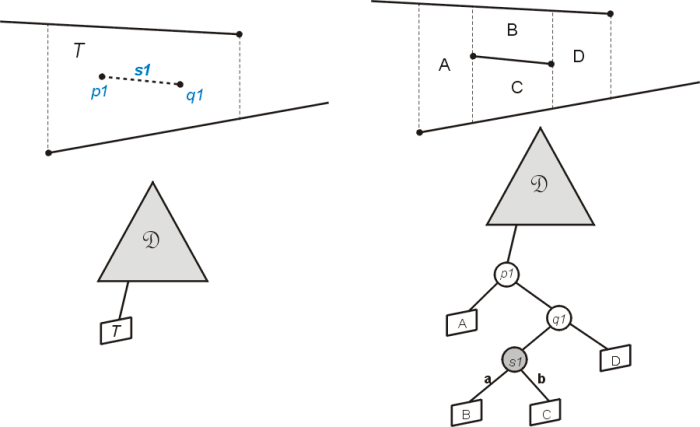
Fig. 3: Inserting a new segment S₁ that falls completely within a single trapezoid (based on de Berg (2000))..

Inserting a Segment Crossing Several Existing Trapezoids

Inserting a segment which crosses several trapezoids is a bit more complicated! Such an insertion is demonstrated in figure 4. In this case four trapezoids T₁, T₁, T₁, and T₁ are deleted and replace by six trapezoids A, B, C, D, E, and F. The first challenge is actually finding the list of trapezoids intersected by s₁. Fortunately the nature of the trapezoid map makes this a relatively straight forward proceedure. Starting with the leftmost point on a line segment we can find the first intersected trapezoid easily by a point query in D. Then we can use the adjacency of trapezoids to find the right neighbour trapezoid into which the segment passes. Segments are assumed to be non-intersecting so we will always cross into an adjacent trapezoid along a vertical extension (if this is not the case then we can always crash the program and send an error report to Microsoft). If the current trapezoid has upper and lower neighbours then this indicates that the right vertical edge is a result of a segment endpoint abutting the current trapezoid, so we need to wether s₁ is above or below rightp(t) of the current trapezoid to determine if we will go to the upper right, or lower right adjacent trapezoid next. This process is repeated until we arrive at the trapezoid containing the segments right endpoint, at which time we have all trapezoids selected. New trapezoids are now formed by adding new vertical extensions to s₁'s endpoints, and shrinking the vertical extensions of the deleted trapezoids to meet s₁ either from above or below, depending on whether their defining point falls below or above s₁.

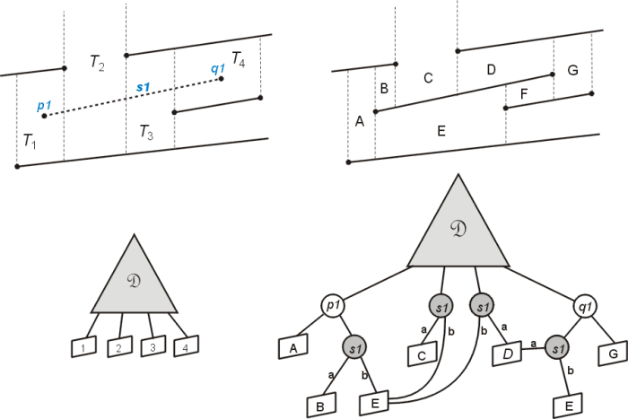
Fig. 4: Inserting a new segment S₁ that spans several trapezoids in the existing trapezoid map.

Updating the search structure is also somewhat involved. The deleted trapezoid nodes are replaced with new sub-trees. The rightmost trapezoid is replaced by a tree rooted at the x-node for p₁, with the new trapezoid A as its left child and a y-node for s₁ as its right child. Trapezoid's B and E are above and below s₁ adjacent to p₁ so their leaf nodes become the above and below children of s₁ respectively. The rightmost endpoint results in a similar situation, with q₁ forming the root and trapezoid G being the right child. For the two trapezoids to the left of q₁ we must test if they are above or below s₁ so a y-node is inserted as q₁'s left child. Updating the pointers for the interior trapezoids T₂ and T₃. We simply need a single y-node for s₁ to test if the trapezoid is above or below the new segment. Finally, we need to take care to child pointers of the y-nodes inserted for s₁ point to the correct child, and we need to updated trapezoid adjacencies, and we are done!

Analysis

Query time for searches in D are linear for the path searched in D to find the trapezoid. Thus the maximum depth of D is of importance. Since each sub-tree added may have a hieght of 3, the worst-case performance is a query time of 3n for a query. However what we are interested in is tthe bound on the average expected query time for the n! possible search structures resulting from all possible random ordering of segment insertions. The analysis, which is quite involved is covered in de Berg(2000) and also in the project of Jukka Kaartien. The expected query time is indeed O(log n). Again the search structure size can be quadratic in the worst case, but he expected size is O(n).